1. Outliers e.g., 
This is further reading for detecting outliers, adopted from http://www.ats.ucla.edu/stat/spss/webbooks/reg/chapter2/spssreg2.htm .
get file = "DirectoryOfYourComputer\crime.sav".

descriptives
  /var=crime murder pctmetro pctwhite pcths poverty single.
		Descriptive Statistics
			N	Minimum	Maximum	Mean	Std. Deviation
violent crime rate	51	82	2922	612.84	441.100
murder rate		51	1.60	78.50	8.7275	10.71758
pct metropolitan	51	24.00	100.00	67.3902	21.95713
pct white		51	31.80	98.50	84.1157	13.25839
pct hs graduates	51	64.30	86.60	76.2235	5.59209
pct poverty		51	8.00	26.40	14.2588	4.58424
pct single parent	51	8.40	22.10	11.3255	2.12149
Valid N (listwise)	51
graph
  /scatterplot(matrix)=crime murder pctmetro pctwhite pcths poverty single .
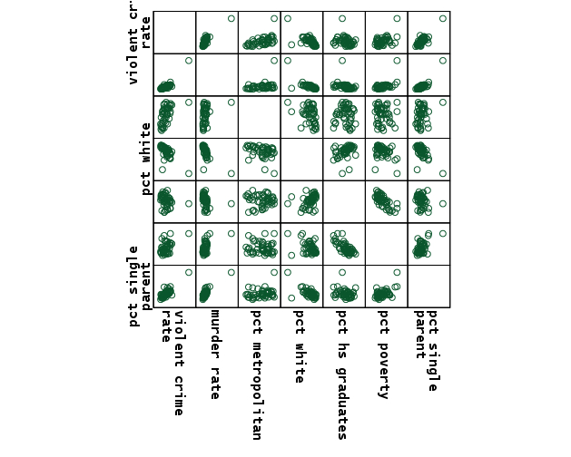
scatterplot for all variables [JPG image (141.43 KB)]
GRAPH /SCATTERPLOT(BIVAR)=pctmetro WITH crime BY state(name) .
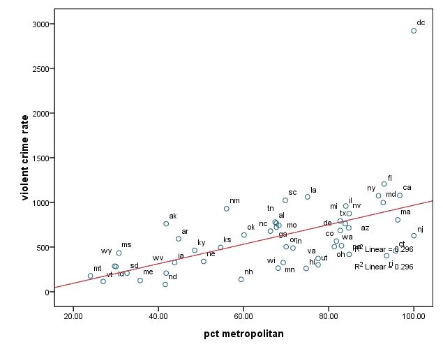
scatterplot of pcmetro by crime by state [JPG image (24.93 KB)]
GRAPH /SCATTERPLOT(BIVAR)=poverty WITH crime BY state(name) .
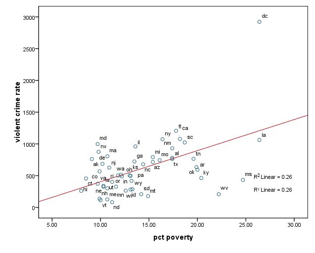
scatterplot of poverty by state [JPG image (23.89 KB)]
GRAPH /SCATTERPLOT(BIVAR)=single WITH crime BY state(name) .
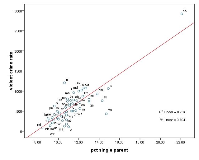
scatterplot of single by state [JPG image (26.6 KB)]
regression
  /dependent crime
  /method=enter pctmetro poverty single.
		Model Summary
Model	R	R Square	Adjusted R Square	Std. Error of the Estimate
1	.916a	.840	.830	182.068
a. Predictors: (Constant), pct single parent, pct metropolitan, pct poverty

			ANOVA(b)
Model			Sum of Squares	df	Mean Square	F	Sig.
1	Regression	8170480.211	3	2723493.404	82.160	.000a
	Residual	1557994.534	47	33148.820
	Total		9728474.745	50
a. Predictors: (Constant), pct single parent, pct metropolitan, pct poverty
b. Dependent Variable: violent crime rate

			Coefficients(a)
		Unstandardized Coefficients		Standardized Coefficients
Model				B		Std. Error	Beta	t	Sig.
1	(Constant)		-1666.436	147.852			-11.271	.000
	pct metropolitan	7.829		1.255		.390	6.240	.000
	pct poverty		17.680		6.941		.184	2.547	.014
	pct single parent	132.408		15.503		.637	8.541	.000
a. Dependent Variable: violent crime rate
regression
  /dependent crime
  /method=enter pctmetro poverty single
  /residuals=histogram.
		Model Summary(b)
Model	R	R Square	Adjusted R Square	Std. Error of the Estimate
1	.916a	.840	.830	182.068
a. Predictors: (Constant), pct single parent, pct metropolitan, pct poverty
b. Dependent Variable: violent crime rate

			ANOVA(b)
Model			Sum of Squares	df	Mean Square	F	Sig.
1	Regression	8170480.211	3	2723493.404	82.160	.000a
	Residual	1557994.534	47	33148.820
	Total		9728474.745	50
a. Predictors: (Constant), pct single parent, pct metropolitan, pct poverty
b. Dependent Variable: violent crime rate

			Coefficients(a)
		Unstandardized Coefficients		Standardized Coefficients
Model				B		Std. Error	Beta	t	Sig.
1	(Constant)		-1666.436	147.852		-11.271	.000
	pct metropolitan	7.829		1.255		.390	6.240	.000
	pct poverty		17.680		6.941		.184	2.547	.014
	pct single parent	132.408		15.503		.637	8.541	.000
a. Dependent Variable: violent crime rate

		Residuals Statistics(a)
			Minimum		Maximum		Mean	Std.Deviation	N
Predicted Value	-30.51		2509.43		612.84	404.240		51
Residual		-523.013	426.111		.000	176.522		51
Std. Predicted Value	-1.592		4.692		.000	1.000		51
Std. Residual		-2.873		2.340		.000	.970		51
a. Dependent Variable: violent crime rate
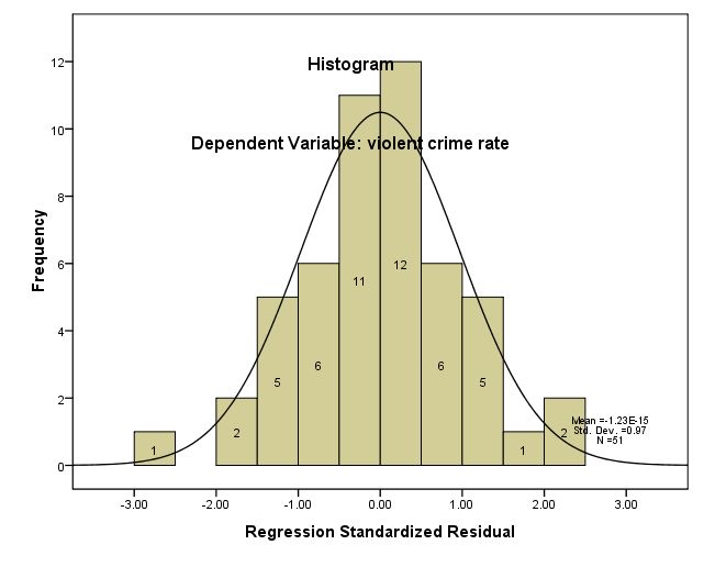
histogram [JPG image (26.38 KB)]
regression
  /dependent crime
  /method=enter pctmetro poverty single
  /residuals=histogram(sdresid).
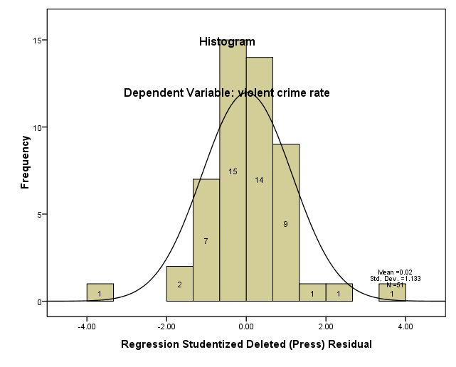
histogram sdresid [JPG image (25.2 KB)]
regression
  /dependent crime
  /method=enter pctmetro poverty single
  /residuals=histogram(sdresid) id(state) outliers(sdresid).
see at http://www2.bc.edu/~stevenw/MB875/mb875_Analyzing Residuals.htm for sdresid (studentized deleted residuals).
		Residuals Statistics(a)
					Minimum		Maximum		Mean	Std. Deviation	N
Predicted Value				-30.51		2509.43		612.84	404.240		51
Std. Predicted Value			-1.592		4.692		.000	1.000		51
Standard Error of Predicted Value	25.788		133.343		47.561	18.563		51
Adjusted Predicted Value		-39.26		2032.11		605.66	369.075		51
Residual				-523.013	426.111		.000	176.522		51
Std. Residual				-2.873		2.340		.000	.970		51
Stud. Residual				-3.194		3.328		.015	1.072		51
Deleted Residual			-646.503	889.885		7.183	223.668		51
Stud. Deleted Residual		-3.571		3.766		.018	1.133		51
Mahal. Distance			.023		25.839		2.941	4.014		51
Cook's Distance			.000		3.203		.089	.454		51
Centered Leverage Value		.000		.517		.059	.080		51
a. Dependent Variable: violent crime rate
regression
  /dependent crime
  /method=enter pctmetro poverty single
  /residuals=histogram(sdresid) id(state) outliers(sdresid)
  /casewise=plot(sdresid) outliers(2)  .
		Casewise Diagnostics(a)
Case Number	state	Stud. Deleted 	violent crime 	Predicted 	Residual
			Residual	rate		Value
9		fl	2.620		1206		779.89		426.111
25		ms	-3.571		434		957.01		-523.013
51		dc	3.766		2922		2509.43		412.566
a. Dependent Variable: violent crime rate
regression
  /dependent crime
  /method=enter pctmetro poverty single
  /residuals=histogram(sdresid lever) id(state) outliers(sdresid lever)
  /casewise=plot(sdresid) outliers(2).
		Outlier Statistics(a)
				Case 	state	Statistic
				Number
Stud. Deleted Residual	1	51	dc 	3.766
			2	25	ms 	-3.571
			3	9	fl 	2.620
			4	18	la 	-1.839
			5	39	ri 	-1.686
			6	12	ia 	1.590
			7	47	wa 	-1.304
			8	13	id 	1.293
			9	14	il 	1.152
			10	35	oh 	-1.148
Centered Leverage Value	1	51	dc 	.517
			2	1	ak 	.241
			3	25	ms 	.171
			4	49	wv 	.161
			5	18	la 	.146
			6	46	vt 	.117
			7	9	fl 	.083
			8	26	mt 	.080
			9	31	nj 	.075
			10	17	ky 	.072
a. Dependent Variable: violent crime rate

histogram sdresid [JPG image (25.2 KB)]
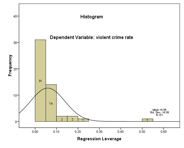
histogram leverage [JPG image (20.5 KB)]
regression
  /dependent crime
  /method=enter pctmetro poverty single
  /residuals=histogram(sdresid lever) id(state) outliers(sdresid, lever)
  /casewise=plot(sdresid)  outliers(2)
  /scatterplot(*lever, *sdresid).
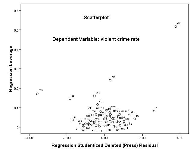
histogram sdresid [JPG image (26.07 KB)]
regression
  /dependent crime
  /method=enter pctmetro poverty single
  /residuals=histogram(sdresid lever) id(state) outliers(sdresid, lever, cook)
  /casewise=plot(sdresid)  outliers(2) cook dffit
  /scatterplot(*lever, *sdresid).
		Casewise Diagnostics(a)
Case Number	state	Stud. 		violent 	Cook's		DFFIT
			Deleted		crime		Distance
			Residual	rate
9	fl		2.620		1206		.174		48.507
25	ms		-3.571		434		.602		-123.490
51	dc		3.766		2922		3.203		477.319
a. Dependent Variable: violent crime rate

		Outlier Statistics(a)
		Case Number	state	Statis	Sig. F
Stud.  		1	51	dc 	3.766
Deleted		2	25	ms 	-3.571
Residual	3	9	fl 	2.620
		4	18	la 	-1.839
		5	39	ri 	-1.686
		6	12	ia 	1.590
		7	47	wa 	-1.304
		8	13	id 	1.293
		9	14	il 	1.152
		10	35	oh 	-1.148
Cook's 		1	51	dc 	3.203	.021
Distance	2	25	ms 	.602	.663
		3	9	fl 	.174	.951
		4	18	la 	.159	.958
		5	39	ri 	.041	.997
		6	12	ia 	.041	.997
		7	13	id 	.037	.997
		8	20	md 	.020	.999
		9	6	co 	.018	.999
		10	49	wv 	.016	.999
Centered  	1	51	dc 	.517
Leverage	2	1	ak 	.241
Value		3	25	ms 	.171
		4	49	wv 	.161
		5	18	la 	.146
		6	46	vt 	.117
		7	9	fl 	.083
		8	26	mt 	.080
		9	31	nj 	.075
		10	17	ky 	.072
a. Dependent Variable: violent crime rate
regression
  /dependent crime
  /method=enter pctmetro poverty single
  /residuals=histogram(sdresid lever) id(state) outliers(sdresid, lever, cook)
  /casewise=plot(sdresid)  outliers(2) cook dffit
  /scatterplot(*lever, *sdresid)
  /save sdbeta(sdfb).
list
  /variables state sdfb1 sdfb2 sdfb3
  /cases from 1 to 10.
state       sdfb1       sdfb2       sdfb3

ak        -.10618     -.13134      .14518
al         .01243      .05529     -.02751
ar        -.06875      .17535     -.10526
az        -.09476     -.03088      .00124
ca         .01264      .00880     -.00364
co        -.03705      .19393     -.13846
ct        -.12016      .07446      .03017
de         .00558     -.01143      .00519
fl         .64175      .59593     -.56060
ga         .03171      .06426     -.09120


Number of cases read:  10    Number of cases listed:  10
VARIABLE LABLES sdfb1 "Sdfbeta pctmetro"
                              /sdfb2 "Sdfbeta poverty"
                              /sdfb3 "Sdfbeta single" .

GRAPH
  /SCATTERPLOT(OVERLAY)=sid sid sid  WITH sdfb1 sdfb2 sdfb3 (PAIR) BY state(name)
  /MISSING=LISTWISE .
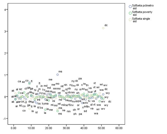
dbfBeta value [JPG image (33.11 KB)]
| Note | |
| Measure | Value |
| leverage | >(2k+2)/n |
| abs(rstu) | > 2 |
| Cook's D | > 4/n |
| abs(DFBETA) | > 2/sqrt(n) |
PRED
Unstandardized predicted values.
RESIDUnstandardized residuals.
DRESIDDeleted residuals.
ADJPREDAdjusted predicted values.
ZPREDStandardized predicted values.
ZRESIDStandardized residuals.
SRESIDStudentized residuals.
SDRESIDStudentized deleted residuals.
SEPREDStandard errors of the predicted values.
MAHALMahalanobis distances.
COOKCook’s distances.
LEVERCentered leverage values.
DFBETAChange in the regression coefficient that results from the deletion of the ith case. A DFBETA value is computed for each case for each regression coefficient generated by a model.
SDBETAStandardized DFBETA. An SDBETA value is computed for each case for each regression coefficient generated by a model.
DFFITChange in the predicted value when the ith case is deleted.
SDFITStandardized DFFIT.
COVRATIORatio of the determinant of the covariance matrix with the ith case deleted to the determinant of the covariance matrix with all cases included.
MCINLower and upper bounds for the prediction interval of the mean predicted response. A lowerbound LMCIN and an upperbound UMCIN are generated. The default confidence interval is 95%. The confidence interval can be reset with the CIN subcommand. (See Dillon & Goldstein
ICINLower and upper bounds for the prediction interval for a single observation. A lowerbound LICIN and an upperbound UICIN are generated. The default confidence interval is 95%. The confidence interval can be reset with the CIN subcommand. (See Dillon & Goldstein
regression
  /dependent crime
  /method=enter pctmetro poverty single
  /residuals=histogram(sdresid lever) id(state) outliers(sdresid, lever, cook)
  /casewise=plot(sdresid)  outliers(2) cook dffit
  /scatterplot(*lever, *sdresid)
  /partialplot.
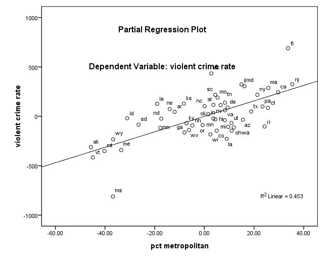
[JPG image (28.2 KB)]
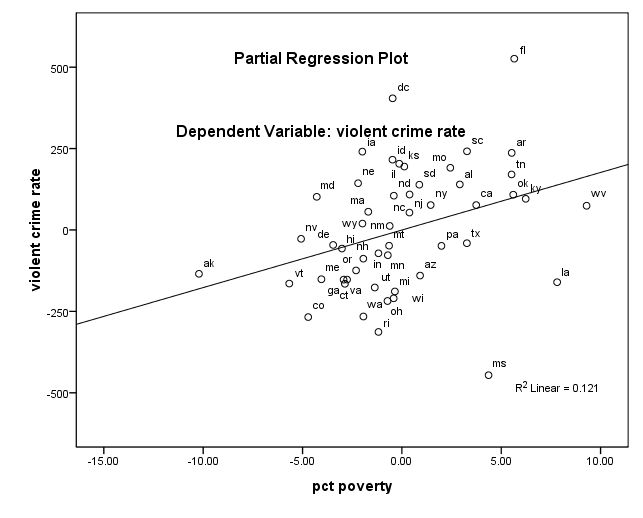
[JPG image (28.53 KB)]
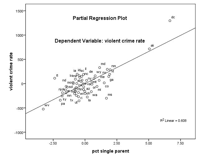
[JPG image (27.35 KB)]
regression
  /dependent crime
  /method=enter pctmetro poverty single.
			Coefficients(a)
		Unstandardized Coefficients		Standardized Coefficients
Model		B	Std. Error	Beta	t	Sig.
1	(Constant)	-1666.436	147.852		-11.271	.000
	pct metropolitan	7.829	1.255	.390	6.240	.000
	pct poverty	17.680	6.941	.184	2.547	.014
	pct single parent	132.408	15.503	.637	8.541	.000
a. Dependent Variable: violent crime rate
compute filtvar = (state NE "dc").
filter by filtvar.
regression
  /dependent crime
  /method=enter pctmetro poverty single .
			Coefficients(a)
		Unstandardized Coefficients		Standardized Coefficients
Model		B	Std. Error	Beta	t	Sig.
1	(Constant)	-1197.538	180.487		-6.635	.000
	pct metropolitan	7.712	1.109	.565	6.953	.000
	pct poverty	18.283	6.136	.265	2.980	.005
	pct single parent	89.401	17.836	.446	5.012	.000
a. Dependent Variable: violent crime rate
2. e.g., 2 
redirected from . . . multiple regression.
 elemapi2.sav (28.49 KB)
 r.api00.OutlierDetection.sps (1.24 KB)
 elemapi2.sav (28.49 KB)
 r.api00.OutlierDetection.sps (1.24 KB)
2.1. inspection 
descriptives /var= ALL .
| Descriptive Statistics | ||||||
| N | Minimum | Maximum | Mean | Std. Deviation | ||
| api 2000 | 400 | 369 | 940 | 647.62 | 142.249 | |
| english language learners | 400 | 0 | 91 | 31.45 | 24.839 | |
| avg class size k-3 | 398 | 14 | 25 | 19.16 | 1.369 | |
| avg parent ed | 381 | 1.00 | 4.62 | 2.6685 | .76379 | |
| pct free meals | 400 | 0 | 100 | 60.32 | 31.912 | |
| Valid N (listwise) | 379 | |||||
graph
  /scatterplot(matrix)=api00 ell acs_k3 avg_ed meals .
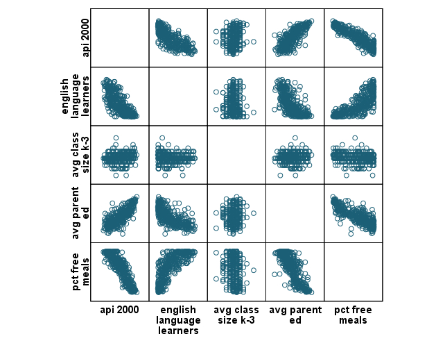
[JPG image (167.94 KB)]
This graph does not give any suspicious cases.
GRAPH /SCATTERPLOT(BIVAR)=ell with api00 .
GRAPH /SCATTERPLOT(BIVAR)=acs_k3 with api00  .
GRAPH /SCATTERPLOT(BIVAR)=avg_ed with api00 .
GRAPH /SCATTERPLOT(BIVAR)=meals with api00  .
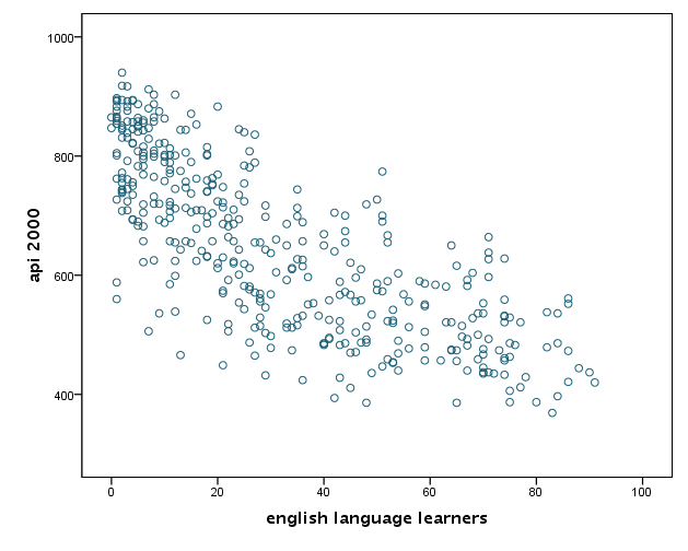 ell [JPG image (129.45 KB)] | 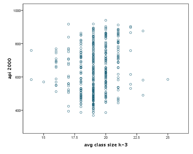 acsk3 [JPG image (77.27 KB)] |
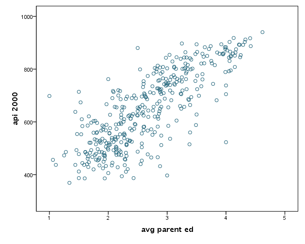 ave_ed [JPG image (117.17 KB)] | 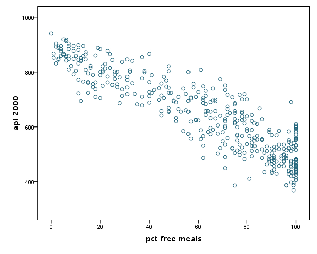 meals [JPG image (119.43 KB)] |
We speculate that the second IV (average class size) is not quite related to DV (api00). And, there seems no particular suspicious data.
REGRESSION
  /DEPENDENT api00
  /METHOD=ENTER ell acs_k3 avg_ed meals
   /residuals=histogram(sdresid lever) id(snum) outliers(sdresid, lever, cook)
  /casewise=plot(sdresid)  outliers(2) cook dffit
  /scatterplot(*lever, *sdresid)
  /save sdbeta(sdfb)
   /partialplot.
| Model Summary | |||||
| Model | R | R Square | Adjusted R Square | Std. Error of the Estimate | |
| 1 | .912a | .833 | .831 | 58.633 | |
| a. Predictors: (Constant), pct free meals, avg class size k-3, english language learners, avg parent ed | |||||
| ANOVA(b) | |||||||
| Model | Sum of Squares | df | Mean Square | F | Sig. | ||
| 1 | Regression | 6393719.254 | 4 | 1598429.813 | 464.956 | .000a | |
| Residual | 1285740.498 | 374 | 3437.809 | ||||
| Total | 7679459.752 | 378 | |||||
| a. Predictors: (Constant), pct free meals, avg class size k-3, english language learners, avg parent ed | |||||||
| b. Dependent Variable: api 2000 | |||||||
| Coefficients(a) | ||||||||
| Unstandardized Coefficients | Standardized Coefficients | |||||||
| Model | B | Std. Error | Beta | t | Sig. | |||
| 1 | (Constant) | 709.639 | 56.240 | 12.618 | .000 | |||
| english language learners | -.843 | .196 | -.147 | -4.307 | .000 | |||
| avg class size k-3 | 3.388 | 2.333 | .032 | 1.452 | .147 | |||
| avg parent ed | 29.072 | 6.924 | .156 | 4.199 | .000 | |||
| pct free meals | -2.937 | .195 | -.655 | -15.081 | .000 | |||
| a. Dependent Variable: api 2000 | ||||||||
| Casewise Diagnostics(a) | |||||||
| Case Number | school number | Stud. Deleted Residual | api 2000 | Cook's Distance | DFFIT | ||
| 93 | 1497 | 2.170 | 604 | .010 | 1.292 | ||
| 97 | 1539 | 2.230 | 700 | .006 | .826 | ||
| 100 | 1515 | 2.222 | 667 | .005 | .661 | ||
| 105 | 1516 | 2.128 | 597 | .010 | 1.380 | ||
| 135 | 1633 | 2.072 | 584 | .044 | 6.085 | ||
| 188 | 1731 | 2.121 | 719 | .015 | 2.126 | ||
| 203 | 1621 | 2.034 | 717 | .006 | .831 | ||
| 226 | 211 | -3.241 | 386 | .015 | -1.325 | ||
| 227 | 182 | -2.653 | 411 | .005 | -.581 | ||
| 228 | 167 | 2.903 | 774 | .010 | .987 | ||
| 232 | 210 | -2.369 | 432 | .018 | -2.263 | ||
| 234 | 165 | -2.734 | 449 | .019 | -1.997 | ||
| 252 | 3700 | 2.036 | 717 | .013 | 1.878 | ||
| 259 | 3537 | -2.425 | 694 | .012 | -1.436 | ||
| 271 | 3758 | 3.012 | 690 | .022 | 2.108 | ||
| 272 | 3794 | 2.083 | 610 | .010 | 1.400 | ||
| 274 | 3759 | -2.290 | 585 | .069 | -8.646 | ||
| 304 | 4507 | 2.011 | 751 | .013 | 1.917 | ||
| 327 | 4737 | 2.470 | 808 | .012 | 1.447 | ||
| 334 | 4744 | 2.160 | 700 | .005 | .645 | ||
| 346 | 5362 | -2.138 | 487 | .010 | -1.359 | ||
| a. Dependent Variable: api 2000 | |||||||
| Residuals Statistics(a) | |||||||
| Minimum | Maximum | Mean | Std. Deviation | N | |||
| Predicted Value | 449.17 | 910.04 | 647.64 | 130.056 | 379 | ||
| Std. Predicted Value | -1.526 | 2.018 | .000 | 1.000 | 379 | ||
| Standard Error of Predicted Value | 3.218 | 14.681 | 6.496 | 1.780 | 379 | ||
| Adjusted Predicted Value | 449.44 | 909.36 | 647.65 | 130.056 | 379 | ||
| Residual | -187.020 | 173.697 | .000 | 58.322 | 379 | ||
| Std. Residual | -3.190 | 2.962 | .000 | .995 | 379 | ||
| Stud. Residual | -3.201 | 2.980 | .000 | 1.002 | 379 | ||
| Deleted Residual | -188.345 | 175.805 | -.016 | 59.138 | 379 | ||
| Stud. Deleted Residual | -3.241 | 3.012 | .000 | 1.005 | 379 | ||
| Mahal. Distance | .141 | 22.702 | 3.989 | 3.030 | 379 | ||
| Cook's Distance | .000 | .069 | .003 | .006 | 379 | ||
| Centered Leverage Value | .000 | .060 | .011 | .008 | 379 | ||
| a. Dependent Variable: api 2000 | |||||||
| Outlier Statistics(a) | |||||||
| Case Number | school number | Statistic | Sig. F | ||||
| Stud. Deleted Residual | 1 | 226 | 211 | -3.241 | |||
| 2 | 271 | 3758 | 3.012 | ||||
| 3 | 228 | 167 | 2.903 | ||||
| 4 | 234 | 165 | -2.734 | ||||
| 5 | 227 | 182 | -2.653 | ||||
| 6 | 327 | 4737 | 2.470 | ||||
| 7 | 259 | 3537 | -2.425 | ||||
| 8 | 232 | 210 | -2.369 | ||||
| 9 | 274 | 3759 | -2.290 | ||||
| 10 | 97 | 1539 | 2.230 | ||||
| Cook's Distance | 1 | 274 | 3759 | .069 | .997 | ||
| 2 | 135 | 1633 | .044 | .999 | |||
| 3 | 26 | 4299 | .030 | 1.000 | |||
| 4 | 193 | 1952 | .025 | 1.000 | |||
| 5 | 271 | 3758 | .022 | 1.000 | |||
| 6 | 234 | 165 | .019 | 1.000 | |||
| 7 | 232 | 210 | .018 | 1.000 | |||
| 8 | 200 | 1872 | .018 | 1.000 | |||
| 9 | 108 | 1606 | .018 | 1.000 | |||
| 10 | 388 | 4878 | .017 | 1.000 | |||
| Centered Leverage Value | 1 | 274 | 3759 | .060 | |||
| 2 | 37 | 4308 | .058 | ||||
| 3 | 209 | 1795 | .050 | ||||
| 4 | 135 | 1633 | .046 | ||||
| 5 | 26 | 4299 | .040 | ||||
| 6 | 69 | 3000 | .037 | ||||
| 7 | 372 | 6068 | .036 | ||||
| 8 | 30 | 4317 | .035 | ||||
| 9 | 147 | 1709 | .035 | ||||
| 10 | 193 | 1952 | .033 | ||||
| a. Dependent Variable: api 2000 | |||||||
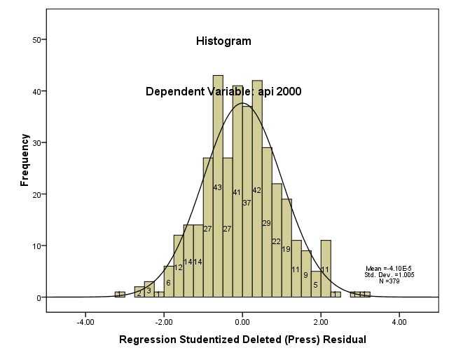
sdresidual check [JPG image (29.53 KB)]
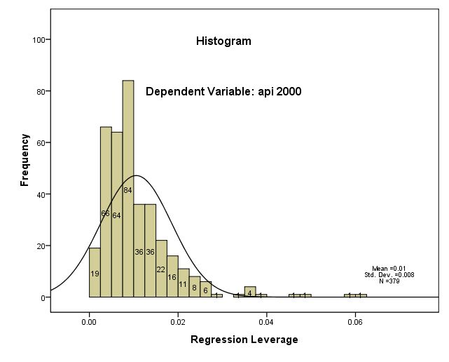
leverage check [JPG image (22.84 KB)]
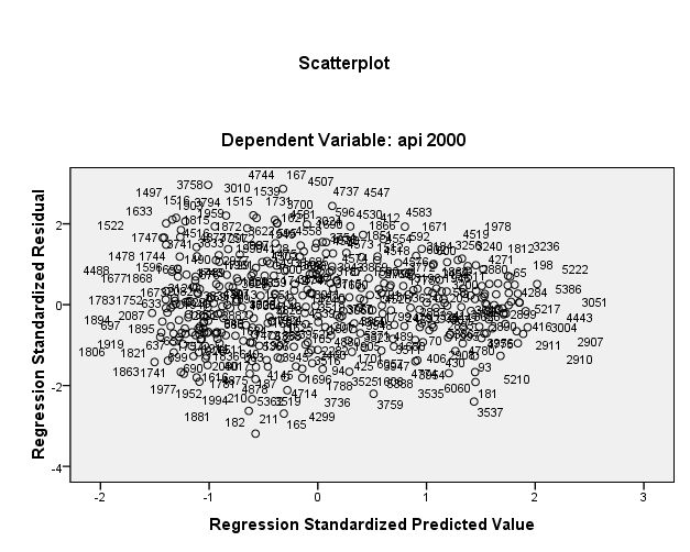
"plot spred by sresid [JPG image (62.22 KB)]
2.2. Outlier dection 
Let's say, we decide to opt out cases whose studentized deleted residual value exceed normal. We set the criterion as ABS(sdresid) > 2. These cases which meet this criterion will filtered out.
We need to save some residual statistics first, with regression method. Saved values include:
PRED
ZPRED
MAHAL
COOK
LEVER
RESID
ZRESID
SDRESID
DFBETA
Among them, we take a look at SDRESID, whose variable name will be SDR_1 in spss data set.ZPRED
MAHAL
COOK
LEVER
RESID
ZRESID
SDRESID
DFBETA
For the referece,
| Note: outlier detection | ||
| Measure | Value | |
| leverage | >(2k+2)/n | 0.021108179 |
| abs(rstu) | > 2 | 2 |
| Cook's D | > 4/n | 0.01055409 |
| abs(DFBETA) | > 2/sqrt(n) | 0.102733099 |
REGRESSION
  /DESCRIPTIVES MEAN STDDEV CORR SIG N
  /MISSING LISTWISE
  /STATISTICS COEFF OUTS R ANOVA COLLIN TOL CHANGE ZPP
  /CRITERIA=PIN(.05) POUT(.10)
  /NOORIGIN
  /DEPENDENT api00
  /METHOD=ENTER meals ell acs_k3 avg_ed
  /residuals=histogram(sdresid lever) id(snum) outliers(sdresid, lever, cook) Durbin
  /casewise=plot(sdresid)  outliers(2) cook dffit
  /SCATTERPLOT=(*ZRESID ,*ZPRED)
  /SAVE PRED ZPRED MAHAL COOK LEVER RESID ZRESID SDRESID DFBETA.
Then, we need to filter out cases whose SDR_1 value exceed:
abs(SDR_1) > 2
with the below command.USE ALL. COMPUTE filterVar=(abs(SDR)_1 < 2). FILTER BY filterVar. EXECUTE.
Then, we do regression again, excluding the suspicious cases. But, this time we do not save the residuals.
Compare the ouptput between the previous and this regression.
REGRESSION
  /DESCRIPTIVES MEAN STDDEV CORR SIG N
  /MISSING LISTWISE
  /STATISTICS COEFF OUTS R ANOVA CHANGE ZPP
  /CRITERIA=PIN(.05) POUT(.10)
  /NOORIGIN
  /DEPENDENT api00
  /METHOD=ENTER ell avg_ed acs_k3 meals
  /SCATTERPLOT=(*ZRESID ,*ZPRED) .
| Model Summaryb | |||||||||
| Model | R | R Square | Adjusted R Square | Std. Error of the Estimate | Change Statistics | ||||
| R Square Change | F Change | df1 | df2 | Sig. F Change | |||||
| 1 | .938a | .880 | .879 | 49.914 | .880 | 649.458 | 4 | 353 | .000 |
| ANOVAb | ||||||
| Model | Sum of Squares | df | Mean Square | F | Sig. | |
| 1 | Regression | 6472284.822 | 4 | 1618071.206 | 649.458 | .000a |
| Residual | 879470.664 | 353 | 2491.418 | |||
| Total | 7351755.486 | 357 | ||||
| Coefficientsa | |||||||||
| Model | Unstandardized Coefficients | Standardized Coefficients | t | Sig. | Correlations | ||||
| B | Std. Error | Beta | Zero-order | Partial | Part | ||||
| 1 | (Constant) | 705.495 | 51.072 | 13.814 | .000 | ||||
| ell | -.915 | .170 | -.160 | -5.374 | .000 | -.789 | -.275 | -.099 | |
| avg_ed | 25.661 | 6.061 | .138 | 4.234 | .000 | .809 | .220 | .078 | |
| acs_k3 | 4.452 | 2.127 | .040 | 2.093 | .037 | .204 | .111 | .039 | |
| meals | -3.056 | .171 | -.683 | -17.868 | .000 | -.928 | -.689 | -.329 | |