FrontPage › StandardError
Difference between r1.7 and the current
@@ -5,6 +5,8 @@
특정 숫자, ''n'' 인 샘플들의 평균들을 모아서 그 분포를 보는 것을 Sample Means Distribution 혹은 Sampling Distribution (샘플평균들의 분포) 라고 하여 이에 대해서는 [wiki:SamplingDistribution Sampling Distribution] 에서 자세히 소개하였다.
Before talking about standard error, let's take a brief look at the concept of normal curve and standard deviation.
표준오차 혹은 Standard Error 는 Standard Deviation of Sample Means 혹은 Standard Deviation of Sample Means Distribution 를 줄여서 부르는 단어이다. 따라서 이 용어는 Standard deviation 와 Sample Means Distribution 의 성격을 파악하고 있으면 이해하기 쉽다.
특정 숫자, n 인 샘플들의 평균들을 모아서 그 분포를 보는 것을 Sample Means Distribution 혹은 Sampling Distribution (샘플평균들의 분포) 라고 하여 이에 대해서는 Sampling Distribution 에서 자세히 소개하였다.
Standard deviation again 
Before talking about standard error, let's take a brief look at the concept of normal curve and standard deviation.
Normal Curve and Standard Deviation,  [1]
[1]
 [1]
[1]P(x) = 1 / sqrt(2 pi sigma^2)*e^(-(x-mu)^2/2 sigma^2) P(x) = 1 / sqrt(2 * pi * (3^2)) * (2.817 ^ (-((x-68)^2) / (2*(3^2)))) . . . . dplot formula for distrib. curve with mu=68, sd=3
This is the mathematical formula for a normal curve. It isn't quiet easy to understand, though, is it? But, I want to briefly go over what the signs and symbols mean in this formula. First, some symbols such as  ; and
; and  are numbers. Probably you know what
  means (it is about 3.1416). And
  is about 2.817. Even though they look difficult to read, they are just numbers like "2" found in the same formula. Another kind is
  and
and  . They represent mean and standard deviation. So, if we assume a normally distributed sample whose mean (
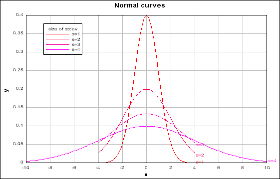
  ) is 0 and standard deviation(
  ) is 1, and draw a graph; it is going to look like the one in the below graph (the highest one). Now remember that we discussed the standard deviation? The formula is (this time, I will show the formula for the variance (
  ):
):
 ; and
; and  are numbers. Probably you know what
  means (it is about 3.1416). And
  is about 2.817. Even though they look difficult to read, they are just numbers like "2" found in the same formula. Another kind is
  and
and  . They represent mean and standard deviation. So, if we assume a normally distributed sample whose mean (
  ) is 0 and standard deviation(
  ) is 1, and draw a graph; it is going to look like the one in the below graph (the highest one). Now remember that we discussed the standard deviation? The formula is (this time, I will show the formula for the variance (
  ):
):
The point was that if the upper part of the formula (the sigma thing) gets big, the stdev -- hence, variance -- will be big. In order for the upper part to be big, the individual sample units (Xi) should be vary a lot from the sample mean (x bar). If the sample units are varying a lot from the mean, the distribution graph should be widely spread.
Now, going back to the normal curve formula, what if standard deviation is 2 and mean is 0? The corresponding graph is the second highest one in the below graphs. I put other graphs whose stdev values are 3 and 4 -- the mean values are 0 for all cases. As you see, the larger is the stdev value, the more spread the corresponding graph is.

[JPG image (83.53 KB)]
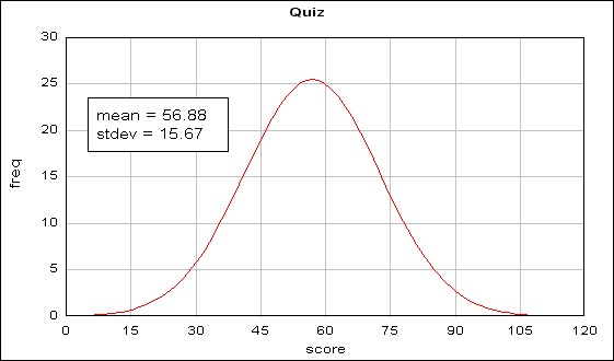
So, if we draw a normal distribution curve of which mean is 56.88 and stdev is 15.67, the graph should look like the below.

[JPG image (31.35 KB)]
Standard Error 
Now let's talk about standard error. Before taking a look at the formula, let's clarify the term standard error. Your immediate response to this term may be error of what? Error for the population parameter -- You know the difference between parameter and statistics, right? The term is slightly out of focus, though it represents what it does very well. The formal name for the standard error should be the standard deviation of sampling distribution (Here, we are back to the concept of standard deviation, again).
There are two kinds of standard errors you need to know.
- The first one is the standard deviation of sampling distribution of
 or "p cap" -- probability.
- The second one is the standard deviation of sampling distribution of mean. The underlying concepts employed here are same. I will focus on the former one, first -- standard deviation of sampling distribution of probability.
1000 people were randomly chosen and 637 answered that they trust the president. So far, the (1) and (2) in the "to-do-list" has been taken care of.
So, the proportion of people who trust the president in your particular sample is:  .
.
 .
.This is what normal people would report when they do survey -- showing percentage. But, it is not enough for you who studied research method. That is, you need do more than this.
That is, what you really want to know is not the  . Rather, you want to know the proportion of the total US citizens, which can be called "
  ."
."
 . Rather, you want to know the proportion of the total US citizens, which can be called "
  ."
."Let's stop here and talk about standard error. But the above will be used again.
The standard deviation of the sampling distribution of  is as follows:
 is as follows:
 and "
and "  " represents sampling statistics (probability), and "
  " represents population parameter (probability). In English, it says that . . .
 - standard deviation of sampling probability (
 )
)
- is equal to
- to
 ,
,  is the sample size
- if you know the proportion (probability) of US citizens' president support,
- you can calculate the standard deviation of your sample's proportion (probability).
Yes!! That is absolutely true. In other words, in the above formula, we DO NOT know the value of  ." But, here is the magic -- it would not be a big problem if we replace
  with
with  obtained from the sample
  , if we are sure that the sample really represents the population, the actual (unknown)
  is about the same as
  .
.
 ." But, here is the magic -- it would not be a big problem if we replace
  with
with  obtained from the sample
  , if we are sure that the sample really represents the population, the actual (unknown)
  is about the same as
  .
. Besides, the value of "  " is relatively insensitive to the changes of
  ." If you look at the below table;
 " is relatively insensitive to the changes of
  ." If you look at the below table;
| p | q | pq | square root (pq) | |
| 0.1 | 0.9 | 0.09 | 0.30 | |
| 0.2 | 0.8 | 0.16 | 0.40 | |
| 0.3 | 0.7 | 0.21 | 0.46 | |
| 0.4 | 0.6 | 0.24 | 0.49 | note that the values here are not much different as found in p and q |
| 0.5 | 0.5 | 0.25 | 0.50 | |
| 0.6 | 0.4 | 0.24 | 0.49 | |
| 0.7 | 0.3 | 0.21 | 0.46 | |
| 0.8 | 0.2 | 0.16 | 0.40 | |
| 0.9 | 0.1 | 0.09 | 0.30 |
- Note that values of
 (column, q) is determined by
  . Suppose that we got 0.6 from sample probability (
  ) and use it as population probability (
  ). Further, suppose that the real value of population probability is 0.5. Then, what is the difference between the calculation -- 0.01. (0.6 * 0.4) vs. (0.5 * 0.5).
 with your
  and assume that the result is not going to be much different. Hence the standard deviation of the sampling distribution is:
 , where
  is sample size.
The left part is called what? standard deviation of the sampling distribution.
- We know what standard deviation means.
- Sampling distribution? not clear . . . (I will be writing about this soon). But, briefly
- If we take a sample (size, n = 1000); measure the probability of the sample and record it; and
- repeat the above step again and again for many many times,
- we get a kind of distribution curve, of which shape is normal.
- If we take a look at this distribution, we will find
- the mean of it (the most frequently appearing probabilities) will be the same as the population probability; and
- the standard deviation of it should be 0.03 (from the above calculation).
- Keeping it in mind that the distribution curve is obtained from the above step 1 and 2 -- sample probabilities,
- we realize that the chance of getting a particular sample probability will follow this distribution.
- That is, if we take one sample, we are coming back to standard deviation rule here,
- 68 out of 100 cases, the sample probability should be found in between the probability of the above distribution PLUS/MINUS ONE standard deviation.
- 95 out of 100 cases, the sample probability should be found in between the probability of the above distribution PLUS/MINUS TWO standard deviation.
- 99 out of 100 cases, the sample probability should be found in between the probability of the above distribution PLUS/MINUS THREE standard deviation.
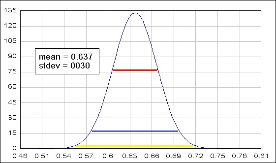
The below is a graphical illustration of it. I am repeating it, here. The distribution curve is obtained from many many sample probabilities. If we take one sample, the chance of getting the sample probability depends on this below distribution curve.

[JPG image (39.74 KB)]
That is,
mean (+-) 1stdev : 0.607 to 0.667   ---   red line = 68%
mean (+-) 2stdev : 0.577 to 0.697   ---  blue line = 95%
mean (+-) 3stdev : 0.547  to 0.727  ---  yellow = 99%
Now carefully think about what you have gotten from your sample statistics. You took a sample whose size is 1000. The purpose of this was not seeing the sample statistics, but, to estimate the population parameters. That's why you carefully (though, the procedures were omitted in this discussion) did random sampling -- to make your random sample representative to the population. Then, you calculated standard deviation of sampling distribution (standard error). This very thing (standard error) is supposed to show how the sample means are distributed if you keep taking samples and getting the means (proportions, in this case). In other words, (this distinction is important!), the standard error is not about your sample itself. It is something about possible means from "many samples (you did not take many samples though; you took only one)." To put this differently, you took a random sample and believed that the sample represents the population. From the statistics you got from the sample, you calculated a number, called standard error.
And, since the standard error is really the standard deviation of sampling distributions, you can employ the idea of guessing game.
That is,
- your sample probability (acquired from the sample you took first place) +- one standard error has about 68% of chance of having the true population probability.
- The sample probability +- two standard deviation has about 95% chance of having the true population probability.
- The sample probability +- three standard deviation has about 99% chance of having the true population probability.
| mean (+-) 1sd: | 0.607 to 0.667 | red line = 68% |
| mean (+-) 2sd: | 0.577 to 0.697 | blue line = 95% |
| mean (+-) 3sd: | 0.547 to 0.727 | yellow = 99% |
Now, you think that the first option 0.607-0.667 cannot be chosen, because the certainty about the true mean of the population is merely 68%. But, it may look cool to say that the true mean resides between 0.607 and 0.667 -- because this is the narrowest range of your guess. But, if you want to do this, you also need to address that you have (only) 68% certainty on your claim. This will not give you a credibility. You don't want to be blamed that you spent the research money for the about half-true (68%) guess. How about choosing the last option (0.547 to 0.727). It has reversed dilemma, now! You may look cool saying that you have 99% of certainty of your claim. But the claim itself has the widest range of possible true mean point (0.547 to 0.727). So, you decide to choose the middle option. I have 95% about the claim that the true mean is in between 0.577-0.697. It seems to be compromising the first and the third option.
On tomorrow's newspaper, there will be a story about your study. The report will say that your firm's research revealed that 63.7% of 1,000 randomly selected people trust the president. From this research, the report will also say, we can use the statistics (63.7%) as the true proportion of the US citizens with plus-minus 6% of error margin.
----


