LiteratureReview › InternetDevelopment › FearAppeal › CompositionTechniques › Project~Twitter_Pattern › AnalyzingSocialNetworks_Borgatti
Difference between r1.79 and the current
@@ -769,16 +769,427 @@
== 7 Visualization ==Data: [attachment:Wiring.zip Roethlisberger & Dickson Bank Wiring Room]
Data: [attachment:Trade.zip Trade data]
Data: [attachment:Campnet.zip Campnet data set] as in Ch. 2
[[Attachment(7-2_Figure-Netdraw.jpg,width=500,caption="Netdraw output")]]
!NetDraw Layout -> Attributes at coordinates[[Attachment(7-4_Figure-MDS.jpg,width=500,caption="MDS")]]
!NetDraw Lighting bolt button
== 8 Testing Hypotheses =='''Permutation'''
. . . So you correlate the variables using your sample data, and get a value like 0.384. The classical significance test then tells you the probability of obtaining a correlation that large given that in the population the variables are actually independent (correlation zero). When this probability is really low (less than 0.05), we call it significant and are willing to claim that the variables are actually related in the population, and not just in your sample.
{{{QAP CORRELATION
--------------------------------------------------------------------------------
Data Matrices: PADGB
PADGM
# of Permutations: 5000
Random seed: 1
Method: Fast: no missing values allowed
QAP results for PADGM * PADGB (5000 permutations)
1 2 3 4 5 6 7 8
Obs Value Significa Average Std Dev Minimum Maximum Prop >= O Prop <= O
--------- --------- --------- --------- --------- --------- --------- ---------
Pearson Correlation 0.3719 0.0008 -0.0004 0.0935 -0.1690 0.4395 0.0008 0.9998
QAP Correlations
1 2
PADGB PADGM
----- -----
1 PADGB 1.000 0.372
2 PADGM 0.372 1.000
QAP P-Values
1 2
PADGB PADGM
----- -----
1 PADGB 0.000 0.001
2 PADGM 0.001 0.000
QAP statistics saved as datafile QAP Correlation Results
----------------------------------------
Running time: 00:00:01
Output generated: 07 10 14 15:15:41
UCINET 6.511 Copyright (c) 1992-2012 Analytic Technologies
}}}
{{{MULTIPLE REGRESSION QAP VIA DOUBLE DEKKER SEMI-PARTIALLING
--------------------------------------------------------------------------------
# of permutations: 2000
Diagonal valid?: NO
Random seed: 963
Dependent variable: KHTec-ADVICE
Partition variable (if any):
Predicted values: KHTec-ADVICE-mrpred (D:\Users\Hyo\OneDrive\Ucinet\Ch08\KHTec-ADVICE-mrpred
Residual values: KHTec-ADVICE-mrResid (D:\Users\Hyo\OneDrive\Ucinet\Ch08\KHTec-ADVICE-mrResid
Model fit stats: KHTec-ADVICE-mrfit (D:\Users\Hyo\OneDrive\Ucinet\Ch08\KHTec-ADVICE-mrfit
Model coefficients: KHTec-ADVICE-mrcoef (D:\Users\Hyo\OneDrive\Ucinet\Ch08\KHTec-ADVICE-mrcoef
Independent variables: D:\Users\Hyo\OneDrive\Ucinet\Ch08\KHTec-FRIENDSHIP
D:\Users\Hyo\OneDrive\Ucinet\Ch08\KHTec-REPORTS_TO
MODEL FIT
R-Square Adj R-Sqr P-Value Obs Perms
------------ ------------ ------------ ------------ ------------
Model 0.063 0.059 0.000 420 2000
REGRESSION COEFFICIENTS
Un-Stdized Stdized Coef P-value As Large As Small Std Err
------------ ------------ ------------ ------------ ------------ ------------
KHTec-FRIENDSHIP 0.13582 0.11701 0.05097 0.05097 0.94953 0.08288
KHTec-REPORTS_TO 0.47157 0.20177 0.00050 0.00050 1.00000 0.11902
Intercept 0.39694 0.00000 0.00000 0.00000 0.00000 0.00000
-----------------------------------------
Running time: 00:00:01 seconds.
Output generated: 07 10 14 15:13:50
}}}
{{{QAP LOGISTIC REGRESSION
--------------------------------------------------------------------------------
Dependent Variable: KHTec-ADVICE (D:\Users\Hyo\OneDrive\Ucinet\Ch08\KHTec-ADVICE
Independent Variables: D:\Users\Hyo\OneDrive\Ucinet\Ch08\KHTec-FRIENDSHIP
D:\Users\Hyo\OneDrive\Ucinet\Ch08\KHTec-REPORTS_TO
# of permutations: 1000
Random seed: 1873119137
Statistics to track: T-Statistics
Data type: Non-Symmetric (directed)
Predicted values: KHTec-ADVICE-pred (D:\Users\Hyo\OneDrive\Ucinet\Ch08\KHTec-ADVICE-pred
Model fit stats: KHTec-ADVICE-fit (D:\Users\Hyo\OneDrive\Ucinet\Ch08\KHTec-ADVICE-fit
Model coefficients: KHTec-ADVICE-coef (D:\Users\Hyo\OneDrive\Ucinet\Ch08\KHTec-ADVICE-coef
Permutation history: history (D:\Users\Hyo\OneDrive\Ucinet\Ch08\history
Dependent variable: : KHTec-ADVICE
Overall fit of the logistic regression model
1 2 3 4 5
LL R-Sqr Sig Obs Perms
--------- --------- --------- --------- ---------
1 Statistics: -274.073 0.065 0.001 420 1000
1 rows, 5 columns, 1 levels.
LR Coefficients & Permutation Results (T-stats used in permutations)
1 2 3 4 5 6 7 8 9 10 11
Coef OddsRat T Sig Avg Min Max SD P(ge) P(le) Perms
--------- --------- --------- --------- --------- --------- --------- --------- --------- --------- ---------
1 Intercept -0.425 0.654 -3.666 1000
2 KHTec-FRIENDSHIP 0.579 1.785 2.418 0.051 0.023 -1.244 0.948 0.345 0.051 0.950 1000
3 KHTec-REPORTS_TO 3.059 21.306 2.956 0.001 -0.010 -1.521 3.059 0.540 0.001 1 1000
3 rows, 11 columns, 1 levels.
-----------------------------------------
Running time: 00:00:01 seconds.
Output generated: 07 10 14 15:21:24
}}}
''' . . . We shall examine the first two time periods to study reciprocity and transitivity. We are interested to know if new friendship ties formed in Week 1 are a result of reciprocity and/or transitivity of ties formed in week 0. '''
{{{DL
N=17
FORMAT = FULLMATRIX DIAGONAL PRESENT
LEVEL LABELS:
"NEWC0"
DATA:
0 0 0 0 0 0 0 0 0 0 1 0 1 0 0 0 1
0 0 0 1 0 0 1 0 0 0 0 0 0 0 0 1 0
0 0 0 0 0 0 0 0 0 0 1 1 0 0 0 0 1
0 1 0 0 0 0 1 0 0 0 0 0 0 0 0 0 1
0 0 0 0 0 0 0 0 0 0 1 1 0 0 0 0 1
0 0 0 1 0 0 0 1 0 0 0 0 1 0 0 0 0
0 0 0 1 0 0 0 0 0 0 0 1 0 0 0 0 1
0 0 0 0 0 1 0 0 0 1 1 0 0 0 0 0 0
0 0 0 0 0 0 0 0 0 0 1 1 0 0 0 0 1
1 0 0 0 0 0 1 0 0 0 0 0 0 0 1 0 0
0 0 0 0 0 0 0 0 1 0 0 1 0 0 0 0 1
0 0 1 0 0 0 0 0 0 0 1 0 0 0 0 0 1
1 0 0 0 0 1 0 0 0 0 0 0 0 0 1 0 0
0 0 0 0 0 0 1 0 1 1 0 0 0 0 0 0 0
0 0 0 0 1 0 0 0 0 1 1 0 0 0 0 0 0
0 0 0 1 0 0 0 0 1 0 1 0 0 0 0 0 0
0 0 0 1 0 0 0 0 1 0 0 1 0 0 0 0 0
}}}
{{{DL
N=17
FORMAT = FULLMATRIX DIAGONAL PRESENT
LEVEL LABELS:
"NEWC1"
DATA:
0 0 0 0 0 0 0 0 1 0 0 0 1 1 0 0 0
0 0 0 1 0 0 1 0 0 0 0 0 0 0 0 0 1
0 0 0 0 0 0 0 0 0 0 0 1 0 0 1 0 1
0 1 0 0 0 0 0 0 1 0 0 0 0 0 0 0 1
1 0 0 0 0 0 0 0 0 0 0 0 1 0 0 0 1
1 0 0 0 0 0 0 0 1 0 0 0 1 0 0 0 0
0 0 0 1 0 0 0 0 0 0 0 1 0 0 0 0 1
0 0 0 0 0 1 0 0 0 1 0 0 1 0 0 0 0
0 0 0 0 0 0 0 0 0 0 1 0 0 1 0 0 1
1 0 0 0 0 0 1 0 0 0 0 0 1 0 0 0 0
0 0 1 0 0 0 0 0 1 0 0 0 0 0 0 0 1
0 0 1 0 0 0 1 0 1 0 0 0 0 0 0 0 0
1 0 0 0 1 1 0 0 0 0 0 0 0 0 0 0 0
0 0 0 1 0 0 1 0 1 0 0 0 0 0 0 0 0
0 0 1 1 1 0 0 0 0 0 0 0 0 0 0 0 0
0 0 0 0 0 0 0 0 1 0 1 0 0 0 0 0 1
0 0 0 1 1 0 0 0 1 0 0 0 0 0 0 0 0
}}}
{{{TRANSPOSE
--------------------------------------------------------------------------------
Input dataset: NEWC0D (D:\Users\Hyo\OneDrive\Ucinet\Ch08\NewFrat\NEWC0D)
Output dataset: NEWC0D-reciprocity (D:\Users\Hyo\OneDrive\Ucinet\Ch08\NewFrat\NEWC0D-reciprocity)
1 2 3 4 5 6 7 8 9 1 1 1 1 1 1 1 1
- - - - - - - - - - - - - - - - -
1 0 0 0 0 0 0 0 0 0 1 0 0 1 0 0 0 0
2 0 0 0 1 0 0 0 0 0 0 0 0 0 0 0 0 0
3 0 0 0 0 0 0 0 0 0 0 0 1 0 0 0 0 0
4 0 1 0 0 0 1 1 0 0 0 0 0 0 0 0 1 1
5 0 0 0 0 0 0 0 0 0 0 0 0 0 0 1 0 0
6 0 0 0 0 0 0 0 1 0 0 0 0 1 0 0 0 0
7 0 1 0 1 0 0 0 0 0 1 0 0 0 1 0 0 0
8 0 0 0 0 0 1 0 0 0 0 0 0 0 0 0 0 0
9 0 0 0 0 0 0 0 0 0 0 1 0 0 1 0 1 1
10 0 0 0 0 0 0 0 1 0 0 0 0 0 1 1 0 0
11 1 0 1 0 1 0 0 1 1 0 0 1 0 0 1 1 0
12 0 0 1 0 1 0 1 0 1 0 1 0 0 0 0 0 1
13 1 0 0 0 0 1 0 0 0 0 0 0 0 0 0 0 0
14 0 0 0 0 0 0 0 0 0 0 0 0 0 0 0 0 0
15 0 0 0 0 0 0 0 0 0 1 0 0 1 0 0 0 0
16 0 1 0 0 0 0 0 0 0 0 0 0 0 0 0 0 0
17 1 0 1 1 1 0 1 0 1 0 1 1 0 0 0 0 0
Transposed matrix saved as dataset D:\Users\Hyo\OneDrive\Ucinet\Ch08\NewFrat\NEWC0D-reciprocity
----------------------------------------
Running time: 00:00:01
Output generated: 07 10 14 15:41:16
UCINET 6.511 Copyright (c) 1992-2012 Analytic Technologies
}}}
{{{TRANSITIVIZE
--------------------------------------------------------------------------------
1 2 3 4 5 6 7 8 9 10 11 12 13 14 15 16 17
-- -- -- -- -- -- -- -- -- -- -- -- -- -- -- -- --
1 0 0 0 1 0 1 0 0 1 0 1 1 1 0 1 0 1
2 0 0 0 1 0 0 1 0 1 0 1 1 0 0 0 1 1
3 0 0 0 1 0 0 0 0 1 0 1 1 0 0 0 0 1
4 0 1 0 0 0 0 1 0 1 0 0 1 0 0 0 1 1
5 0 0 1 1 0 0 0 0 1 0 1 1 0 0 0 0 1
6 1 1 0 1 0 0 1 1 0 1 1 0 1 0 1 0 1
7 0 1 1 1 0 0 0 0 1 0 1 1 0 0 0 0 1
8 1 0 0 1 0 1 1 0 1 1 1 1 1 0 1 0 1
9 0 0 1 1 0 0 0 0 0 0 1 1 0 0 0 0 1
10 1 0 0 1 1 0 1 0 0 0 1 1 1 0 1 0 1
11 0 0 1 1 0 0 0 0 1 0 0 1 0 0 0 0 1
12 0 0 1 1 0 0 0 0 1 0 1 0 0 0 0 0 1
13 1 0 0 1 1 1 0 1 0 1 1 0 0 0 1 0 1
14 1 0 0 1 0 0 1 0 1 1 1 1 0 0 1 0 1
15 1 0 0 0 1 0 1 0 1 1 1 1 0 0 0 0 1
16 0 1 0 1 0 0 1 0 1 0 1 1 0 0 0 0 1
17 0 1 1 1 0 0 1 0 1 0 1 1 0 0 0 0 0
17 rows, 17 columns, 1 levels.
-----------------------------------------
Running time: 00:00:01 seconds.
Output generated: 07 10 14 15:41:50
UCINET 6.511 Copyright (c) 1992-2012 Analytic Technologies
}}}
{{{QAP LOGISTIC REGRESSION
--------------------------------------------------------------------------------
Dependent Variable: NEWC1D (D:\Users\Hyo\OneDrive\Ucinet\Ch08\NewFrat\NEWC1D
Independent Variables: D:\Users\Hyo\OneDrive\Ucinet\Ch08\NewFrat\NEWC0D
D:\Users\Hyo\OneDrive\Ucinet\Ch08\NewFrat\NEWC0D-reciprocity
D:\Users\Hyo\OneDrive\Ucinet\Ch08\NewFrat\NEWC0D-transitivity
# of permutations: 10000
Random seed: 2058888892
Statistics to track: T-Statistics
Data type: Non-Symmetric (directed)
Predicted values: NEWC1D-pred (D:\Users\Hyo\OneDrive\Ucinet\Ch08\NewFrat\NEWC1D-pred
Model fit stats: NEWC1D-fit (D:\Users\Hyo\OneDrive\Ucinet\Ch08\NewFrat\NEWC1D-fit
Model coefficients: NEWC1D-coef (D:\Users\Hyo\OneDrive\Ucinet\Ch08\NewFrat\NEWC1D-coef
Permutation history: history (D:\Users\Hyo\OneDrive\Ucinet\Ch08\NewFrat\history
Dependent variable: : NEWC1D
Overall fit of the logistic regression model
1 2 3 4 5
LL R-Sqr Sig Obs Perms
---------- ---------- ---------- ---------- ----------
1 Statistics: -100.284 0.263 0.000 272 10000
1 rows, 5 columns, 1 levels.
LR Coefficients & Permutation Results (T-stats used in permutations)
1 2 3 4 5 6 7 8 9 10 11
Coef OddsRat T Sig Avg Min Max SD P(ge) P(le) Perms
---------- ---------- ---------- ---------- ---------- ---------- ---------- ---------- ---------- ---------- ----------
1 Intercept -2.764 0.063 -8.096 10000
2 NEWC0D 1.833 6.253 4.053 0.000 -0.007 -2.592 2.672 0.482 0.000 1.000 10000
3 NEWC0D-reciprocity 0.806 2.239 1.943 0.012 -0.013 -1.868 1.160 0.369 0.012 0.988 10000
4 NEWC0D-transitivity 0.923 2.517 1.982 0.045 0.001 -2.359 1.690 0.433 0.045 0.955 10000
4 rows, 11 columns, 1 levels.
-----------------------------------------
Running time: 00:00:03 seconds.
Output generated: 07 10 14 15:43:42
}}}
== 9 Characterizing Whole Networks ==== 10 Centrality ==
== 11 Subgroups ==
== 12 Equivalence ==
{{{1 2 3 4 5 6 7 8 9 10 11 12 13 14 15 16 17 18
RO BO AM BE PE LO VI WI JO GR HU BO MA AL AM BA EL SI
-- -- -- -- -- -- -- -- -- -- -- -- -- -- -- -- -- --
ROMULAND 0 7 7 8 11 7 8 5 9 10 7 7 8 7 7 9 8 8
BONAVENTURE 7 0 5 8 12 8 7 8 10 12 9 8 9 8 9 11 10 10
AMBROSE 7 5 0 9 12 9 7 7 10 11 8 8 10 8 9 10 10 10
BERTHOLD 8 8 9 0 10 10 9 10 11 12 11 10 9 10 10 10 10 11
PETER 11 12 12 10 0 10 12 12 13 13 12 12 13 13 11 12 12 13
LOUIS 7 8 9 10 10 0 10 8 10 12 10 9 10 9 7 10 10 10
VICTOR 8 7 7 9 12 10 0 8 11 12 10 9 11 9 10 11 10 9
WINFRID 5 8 7 10 12 8 8 0 8 9 6 5 8 7 8 8 9 9
JOHN 9 10 10 11 13 10 11 8 0 10 10 10 11 10 9 11 11 11
GREGORY 10 12 11 12 13 12 12 9 10 0 9 9 11 10 11 9 12 12
HUGH 7 9 8 11 12 10 10 6 10 9 0 5 9 7 9 9 10 9
BONIFACE 7 8 8 10 12 9 9 5 10 9 5 0 7 5 9 9 9 9
MARK 8 9 10 9 13 10 11 8 11 11 9 7 0 6 9 9 9 9
ALBERT 7 8 8 10 13 9 9 7 10 10 7 5 6 0 9 9 9 9
AMAND 7 9 9 10 11 7 10 8 9 11 9 9 9 9 0 9 9 9
BASIL 9 11 10 10 12 10 11 8 11 9 9 9 9 9 9 0 7 9
ELIAS 8 10 10 10 12 10 10 9 11 12 10 9 9 9 9 7 0 5
SIMPLICIUS 8 10 10 11 13 10 9 9 11 12 9 9 9 9 9 9 5 0
}}}
== 13 Analyzing Two-Mode Data ==Davis data
=== 7. Equivalence ===
Use the Davis data
{{{Tools -> Similarities & Distances
}}}
---
{{{input: davis
output: davis-Mat-C
Matches . . . . Cols}}}
---
{{{input: davis
output: davis-Mat-R
Matches . . . . Rows}}}
---
Use the two output files, with the original data file
{{{Network -> Cohesion -> Density with Group
input: davis
row partition: davis-Mat-R
columns partion: davis-Mat-C
}}}
== 15 Ego Networks ==
== References ==
Contents
- 1. 1 Introduction
- 2. 2 Mathematical Foundations
- 3. 3 Research Design
- 4. 4 Data Collection
- 5. 5 Data Management
- 6. 6 Multivariate Techniques Used in Network Analysis
- 7. 7 Visualization
- 8. 8 Testing Hypotheses
- 9. 9 Characterizing Whole Networks
- 10. 10 Centrality
- 11. 11 Subgroups
- 12. 12 Equivalence
- 13. 13 Analyzing Two-Mode Data
- 14. 14 Large Networks
- 15. 15 Ego Networks
- 16. References
- 17. Index
Preface
5. 5 Data Management 
Data management:
----
----
 UCINET_6_Users_Guide.docx (96.48 KB)
 Entering Data Using the DL Editor.docx (432.31 KB)
Learning Outcomes
- Configure network and attribute data for standard software packages
- Apply elementary transformations to matrix data
- Extract and reconfigure network and attribute data
5.1. Introduction 
We will discuss:
![[https]](/imgs/https.png) UCINET.
UCINET.
- how to format network data for import into a network analysis software package,
- how to transform network data to make it suitable for different analyses, and
- how to export network data and results for use in other programs.
![[https]](/imgs/https.png) UCINET.
UCINET. 5.2. Data import 
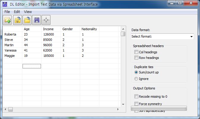
For most users, we recommend using Microsoft Excel as a sort of universal translator (or any kind of spreadsheet program).
And DL format (data language)
UCINET tackles various format such as . . .
- matrix format
- list format
- Nodelist
- Edgelist
- Nodelist
5.2.2. List formats 
- matrix format takes a lot of space in terms of memory and disk.
- Indicating the only relations among the network nodes may be more efficient.
5.2.2.1. Nodelist 
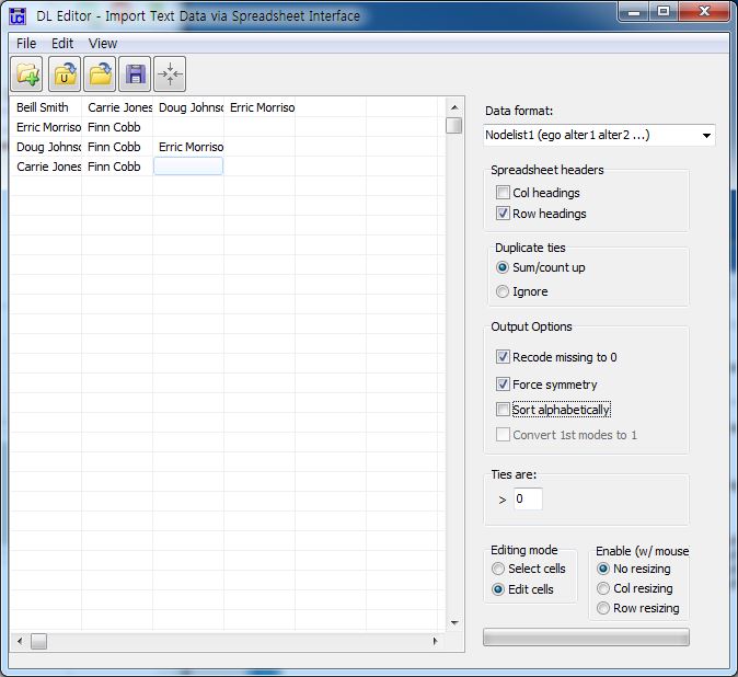 [JPG image (69.46 KB)] |
DL
N=5
FORMAT = FULLMATRIX DIAGONAL PRESENT
SYMMETRIC = YES
LABELS embedded
DATA:
"Beill Smith" "Carrie Jones" "Doug Johnson" "Erric Morrison"
"Erric Morrison" "Finn Cobb"
"Doug Johnson" "Finn Cobb" "Erric Morrison"
"Carrie Jones" "Finn Cobb"
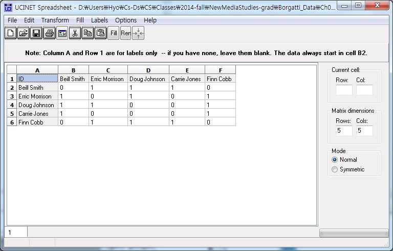 [JPG image (66.1 KB)] |
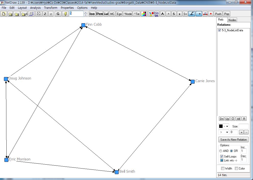 [JPG image (80.2 KB)] |  5-3_NodeListData2.txt (255 Bytes) OR 5-3_NodeListData2.txt (255 Bytes) OR 5-3_NodeListData.txt (749 Bytes) 5-3_NodeListData.txt (749 Bytes) |
| Two mode data |  5-6_TwoModeNodelistDlFile.txt (176 Bytes) 5-6_TwoModeNodelistDlFile.txt (176 Bytes) |
DL nr=3, nc=5
format=nodelist2
row labels embedded
column labels embedded
data:
George, Darts, Pool, Dancing
Sue, Dancing, Volleyball
Sally, Dancing, Darts, Basketball
5.2.2.2. Edgelist 
Each row has two columns indicating the pair of nodes that have the tie. Optionally, a third column can be included which gives the strength of the tie. . . .
| Node1 | Node2 |
| Node1 | Node2 | 3 |
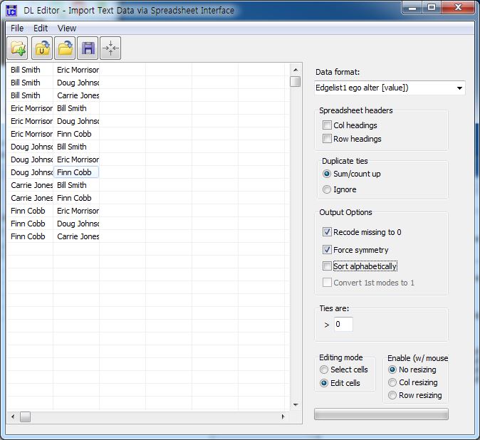
[JPG image (75.92 KB)]
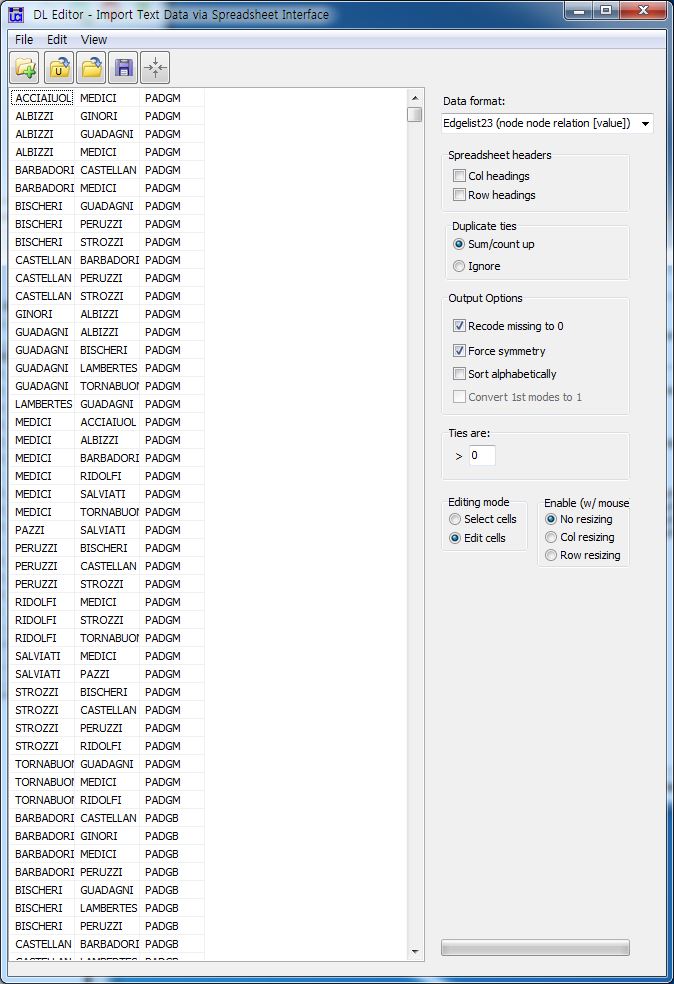
[JPG image (124.18 KB)]
5.3. Cleaning network data 
- Be careful:
replicated actor
missing actor
- Data characteristics
had lunch with . . . . data should be symmetric.
What do you do about it?
- Take a look at isolates.
- Ethnographic hunch . . . Who's gonna be the center . . . Make a quick picture of the data.
5.4. Data transformation 
- transposing matrices,
- symmetrizing,
- dichotomizing,
- imputing missing values,
- combining relations,
- combining nodes,
- extracting subgraphs, and many more.
- Permute: Re-order rows, columns or matrices in a dataset according to a user specified list.
- bipartite: Convert a 2-mode dataset into a 1-mode adjacency matrix
- Any 2-mode incidence matrix can be thought of as a bipartite graph. If the 2-modes are actors and events then the bipartite graph consists of the union of the actors and events as vertices with the edges only connecting actors with events (ie no connections between actors or between events). This routine takes a 2-mode incidence matrix and converts it to a 1-mode adjacency matrix of a bipartite graph. If the incidence matrix had n rows and m columns then the resultant adjacency matrix would be a square matrix of dimension m+n.
- Any 2-mode incidence matrix can be thought of as a bipartite graph. If the 2-modes are actors and events then the bipartite graph consists of the union of the actors and events as vertices with the edges only connecting actors with events (ie no connections between actors or between events). This routine takes a 2-mode incidence matrix and converts it to a 1-mode adjacency matrix of a bipartite graph. If the incidence matrix had n rows and m columns then the resultant adjacency matrix would be a square matrix of dimension m+n.
5.4.1. Transposing 
- To interchange its rows with its columns
- When the matrix is non-symmetric, it makes relationships reversed. (Transposing an adjacency matrix is equivalent to reversing the direction of the arrows.)
- by suvey's nature, it becomes very useful.
- 'who do you seek advice from?' : the constructed data should be transposed:
- food webs, too.
- which species eat which species?
- whose energy flow to whom? = The matrix is transposed by ecologist.
- which species eat which species?
- 'who do you seek advice from?' : the constructed data should be transposed:
- row x col x layers
- row - col
- row - layer
- col - layer
- row - col
- Padgett dataset: marriage and business ties among Florentine families during the Renaissance period.
DL
N=16 NM=2
FORMAT = FULLMATRIX DIAGONAL PRESENT
ROW LABELS:
"ACCIAIUOL"
"ALBIZZI"
"BARBADORI"
"BISCHERI"
"CASTELLAN"
"GINORI"
"GUADAGNI"
"LAMBERTES"
"MEDICI"
"PAZZI"
"PERUZZI"
"PUCCI"
"RIDOLFI"
"SALVIATI"
"STROZZI"
"TORNABUON"
COLUMN LABELS:
"ACCIAIUOL"
"ALBIZZI"
"BARBADORI"
"BISCHERI"
"CASTELLAN"
"GINORI"
"GUADAGNI"
"LAMBERTES"
"MEDICI"
"PAZZI"
"PERUZZI"
"PUCCI"
"RIDOLFI"
"SALVIATI"
"STROZZI"
"TORNABUON"
LEVEL LABELS:
"PADGM"
"PADGB"
DATA:
 0 0 0 0 0 0 0 0 1 0 0 0 0 0 0 0
 0 0 0 0 0 1 1 0 1 0 0 0 0 0 0 0
 0 0 0 0 1 0 0 0 1 0 0 0 0 0 0 0
 0 0 0 0 0 0 1 0 0 0 1 0 0 0 1 0
 0 0 1 0 0 0 0 0 0 0 1 0 0 0 1 0
 0 1 0 0 0 0 0 0 0 0 0 0 0 0 0 0
 0 1 0 1 0 0 0 1 0 0 0 0 0 0 0 1
 0 0 0 0 0 0 1 0 0 0 0 0 0 0 0 0
 1 1 1 0 0 0 0 0 0 0 0 0 1 1 0 1
 0 0 0 0 0 0 0 0 0 0 0 0 0 1 0 0
 0 0 0 1 1 0 0 0 0 0 0 0 0 0 1 0
 0 0 0 0 0 0 0 0 0 0 0 0 0 0 0 0
 0 0 0 0 0 0 0 0 1 0 0 0 0 0 1 1
 0 0 0 0 0 0 0 0 1 1 0 0 0 0 0 0
 0 0 0 1 1 0 0 0 0 0 1 0 1 0 0 0
 0 0 0 0 0 0 1 0 1 0 0 0 1 0 0 0
 0 0 0 0 0 0 0 0 0 0 0 0 0 0 0 0
 0 0 0 0 0 0 0 0 0 0 0 0 0 0 0 0
 0 0 0 0 1 1 0 0 1 0 1 0 0 0 0 0
 0 0 0 0 0 0 1 1 0 0 1 0 0 0 0 0
 0 0 1 0 0 0 0 1 0 0 1 0 0 0 0 0
 0 0 1 0 0 0 0 0 1 0 0 0 0 0 0 0
 0 0 0 1 0 0 0 1 0 0 0 0 0 0 0 0
 0 0 0 1 1 0 1 0 0 0 1 0 0 0 0 0
 0 0 1 0 0 1 0 0 0 1 0 0 0 1 0 1
 0 0 0 0 0 0 0 0 1 0 0 0 0 0 0 0
 0 0 1 1 1 0 0 1 0 0 0 0 0 0 0 0
 0 0 0 0 0 0 0 0 0 0 0 0 0 0 0 0
 0 0 0 0 0 0 0 0 0 0 0 0 0 0 0 0
 0 0 0 0 0 0 0 0 1 0 0 0 0 0 0 0
 0 0 0 0 0 0 0 0 0 0 0 0 0 0 0 0
 0 0 0 0 0 0 0 0 1 0 0 0 0 0 0 0
- centrality measure
MULTIPLE CENTRALITY MEASURES
--------------------------------------------------------------------------------

Input dataset: PADGETT (D:\Users\Hyo\Cs-Ds\CS\Classes\2014-fall\NewMediaStudies-grad\Borgatti_Data\Ch05\PADGETT)
Output dataset: PADGETT-cent (D:\Users\Hyo\Cs-Ds\CS\Classes\2014-fall\NewMediaStudies-grad\Borgatti_Data\Ch05\PADGETT-cent)
Treat data as:                          Auto-detect
Type of scores to output:               Raw scores
Undefined dist in closeness:            replace with max dist + 1

Network PADGM is directed? NO

Value of Beta was:                      0.305579943942584
Network PADGB is directed? NO

Value of Beta was:                      0.300228499969756
Centrality Measures

PADGM

                     1       2       3       4       5       6       7       8       9
                Degree  2local  BonPwr   2Step     ARD Closene Eigenve Between 2StepBe
               ------- ------- ------- ------- ------- ------- ------- ------- -------
  1 ACCIAIUOL    1.000   6.000 301.290   6.000   5.917  44.000   0.132   0.000   0.000
  2   ALBIZZI    3.000  11.000 557.416  10.000   7.833  35.000   0.244  19.333   2.500
  3 BARBADORI    2.000   9.000 482.693   9.000   7.083  38.000   0.212   8.500   1.000
  4  BISCHERI    3.000  11.000 644.632   8.000   7.200  41.000   0.283   9.500   2.000
  5 CASTELLAN    3.000   9.000 590.363   6.000   6.917  42.000   0.259   5.000   2.000
  6    GINORI    1.000   3.000 171.335   3.000   5.333  48.000   0.075   0.000   0.000
  7  GUADAGNI    4.000  10.000 660.285   9.000   8.083  36.000   0.289  23.167   5.500
  8 LAMBERTES    1.000   4.000 202.770   4.000   5.367  49.000   0.089   0.000   0.000
  9    MEDICI    6.000  14.000 982.689  11.000   9.500  31.000   0.430  47.500  13.500
 10     PAZZI    1.000   2.000 102.991   2.000   4.767  55.000   0.045   0.000   0.000
 11   PERUZZI    3.000  10.000 628.266   6.000   6.783  44.000   0.276   2.000   0.500
 12     PUCCI    0.000   0.000  -0.000   0.000   0.000  90.000   0.000   0.000   0.000
 13   RIDOLFI    3.000  13.000 778.167  11.000   8.000  34.000   0.342  10.333   2.000
 14  SALVIATI    2.000   7.000 333.762   7.000   6.583  42.000   0.146  13.000   1.000
 15   STROZZI    4.000  12.000 811.167   8.000   7.833  38.000   0.356   9.333   3.500
 16 TORNABUON    3.000  13.000 742.852  10.000   7.833  35.000   0.326   8.333   1.500


PADGB

                     1       2       3       4       5       6       7       8       9
                Degree  2local  BonPwr   2Step     ARD Closene Eigenve Between 2StepBe
               ------- ------- ------- ------- ------- ------- ------- ------- -------
  1 ACCIAIUOL    0.000   0.000   0.000   0.000   0.000  90.000   0.000   0.000   0.000
  2   ALBIZZI    0.000   0.000   0.000   0.000   0.000  90.000   0.000   0.000   0.000
  3 BARBADORI    4.000  14.000 756.242   9.000   6.833  47.000   0.390  25.000   4.000
  4  BISCHERI    3.000  10.000 663.468   5.000   5.417  55.000   0.344   2.500   0.500
  5 CASTELLAN    3.000  12.000 754.534   7.000   6.000  50.000   0.391   5.000   0.500
  6    GINORI    2.000   9.000 370.702   7.000   5.417  52.000   0.191   0.000   0.000
  7  GUADAGNI    2.000   7.000 452.922   4.000   4.433  62.000   0.235   0.000   0.000
  8 LAMBERTES    4.000  12.000 838.463   5.000   5.917  54.000   0.435   6.000   2.000
  9    MEDICI    5.000   9.000 471.830   7.000   6.917  49.000   0.241  24.000   9.000
 10     PAZZI    1.000   5.000 142.657   5.000   4.367  58.000   0.073   0.000   0.000
 11   PERUZZI    4.000  14.000 908.501   7.000   6.500  49.000   0.471  13.500   2.000
 12     PUCCI    0.000   0.000   0.000   0.000   0.000  90.000   0.000   0.000   0.000
 13   RIDOLFI    0.000   0.000   0.000   0.000   0.000  90.000   0.000   0.000   0.000
 14  SALVIATI    1.000   5.000 142.657   5.000   4.367  58.000   0.073   0.000   0.000
 15   STROZZI    0.000   0.000   0.000   0.000   0.000  90.000   0.000   0.000   0.000
 16 TORNABUON    1.000   5.000 142.657   5.000   4.367  58.000   0.073   0.000   0.000


----------------------------------------
Running time:  00:00:01
Output generated:  29 9 14 16:41:40
UCINET 6.511 Copyright (c) 1992-2012 Analytic Technologies
[1] Degree

                  1 2
                  P P
                  - -
    1  ACCIAIUOL  1 0
    2    ALBIZZI  3 0
    3  BARBADORI  2 4
    4   BISCHERI  3 3
    5  CASTELLAN  3 3
    6     GINORI  1 2
    7   GUADAGNI  4 2
    8  LAMBERTES  1 4
    9     MEDICI  6 5
   10      PAZZI  1 1
   11    PERUZZI  3 4
   12      PUCCI  0 0
   13    RIDOLFI  3 0
   14   SALVIATI  2 1
   15    STROZZI  4 0
   16  TORNABUON  3 1

[2] 2local

                   1  2
                  PA PA
                  -- --
    1  ACCIAIUOL   6  0
    2    ALBIZZI  11  0
    3  BARBADORI   9 14
    4   BISCHERI  11 10
    5  CASTELLAN   9 12
    6     GINORI   3  9
    7   GUADAGNI  10  7
    8  LAMBERTES   4 12
    9     MEDICI  14  9
   10      PAZZI   2  5
   11    PERUZZI  10 14
   12      PUCCI   0  0
   13    RIDOLFI  13  0
   14   SALVIATI   7  5
   15    STROZZI  12  0
   16  TORNABUON  13  5

[3] BonPwr

                        1       2
                    PADGM   PADGB
                  ------- -------
    1  ACCIAIUOL  301.290   0.000
    2    ALBIZZI  557.416   0.000
    3  BARBADORI  482.693 756.242
    4   BISCHERI  644.632 663.468
    5  CASTELLAN  590.363 754.534
    6     GINORI  171.335 370.702
    7   GUADAGNI  660.285 452.922
    8  LAMBERTES  202.770 838.463
    9     MEDICI  982.689 471.830
   10      PAZZI  102.991 142.657
   11    PERUZZI  628.266 908.501
   12      PUCCI   -0.000   0.000
   13    RIDOLFI  778.167  -0.000
   14   SALVIATI  333.762 142.657
   15    STROZZI  811.167   0.000
   16  TORNABUON  742.852 142.657

[4] 2Step

                   1  2
                  PA PA
                  -- --
    1  ACCIAIUOL   6  0
    2    ALBIZZI  10  0
    3  BARBADORI   9  9
    4   BISCHERI   8  5
    5  CASTELLAN   6  7
    6     GINORI   3  7
    7   GUADAGNI   9  4
    8  LAMBERTES   4  5
    9     MEDICI  11  7
   10      PAZZI   2  5
   11    PERUZZI   6  7
   12      PUCCI   0  0
   13    RIDOLFI  11  0
   14   SALVIATI   7  5
   15    STROZZI   8  0
   16  TORNABUON  10  5

[5] ARD

                      1     2
                  PADGM PADGB
                  ----- -----
    1  ACCIAIUOL  5.917 0.000
    2    ALBIZZI  7.833 0.000
    3  BARBADORI  7.083 6.833
    4   BISCHERI  7.200 5.417
    5  CASTELLAN  6.917 6.000
    6     GINORI  5.333 5.417
    7   GUADAGNI  8.083 4.433
    8  LAMBERTES  5.367 5.917
    9     MEDICI  9.500 6.917
   10      PAZZI  4.767 4.367
   11    PERUZZI  6.783 6.500
   12      PUCCI  0.000 0.000
   13    RIDOLFI  8.000 0.000
   14   SALVIATI  6.583 4.367
   15    STROZZI  7.833 0.000
   16  TORNABUON  7.833 4.367

[6] Closeness

                   1  2
                  PA PA
                  -- --
    1  ACCIAIUOL  44 90
    2    ALBIZZI  35 90
    3  BARBADORI  38 47
    4   BISCHERI  41 55
    5  CASTELLAN  42 50
    6     GINORI  48 52
    7   GUADAGNI  36 62
    8  LAMBERTES  49 54
    9     MEDICI  31 49
   10      PAZZI  55 58
   11    PERUZZI  44 49
   12      PUCCI  90 90
   13    RIDOLFI  34 90
   14   SALVIATI  42 58
   15    STROZZI  38 90
   16  TORNABUON  35 58

[7] Eigenvector

                       1      2
                   PADGM  PADGB
                  ------ ------
    1  ACCIAIUOL   0.132  0.000
    2    ALBIZZI   0.244  0.000
    3  BARBADORI   0.212  0.390
    4   BISCHERI   0.283  0.344
    5  CASTELLAN   0.259  0.391
    6     GINORI   0.075  0.191
    7   GUADAGNI   0.289  0.235
    8  LAMBERTES   0.089  0.435
    9     MEDICI   0.430  0.241
   10      PAZZI   0.045  0.073
   11    PERUZZI   0.276  0.471
   12      PUCCI   0.000 -0.000
   13    RIDOLFI   0.342  0.000
   14   SALVIATI   0.146  0.073
   15    STROZZI   0.356 -0.000
   16  TORNABUON   0.326  0.073

[8] Between

                       1      2
                   PADGM  PADGB
                  ------ ------
    1  ACCIAIUOL   0.000  0.000
    2    ALBIZZI  19.333  0.000
    3  BARBADORI   8.500 25.000
    4   BISCHERI   9.500  2.500
    5  CASTELLAN   5.000  5.000
    6     GINORI   0.000  0.000
    7   GUADAGNI  23.167  0.000
    8  LAMBERTES   0.000  6.000
    9     MEDICI  47.500 24.000
   10      PAZZI   0.000  0.000
   11    PERUZZI   2.000 13.500
   12      PUCCI   0.000  0.000
   13    RIDOLFI  10.333  0.000
   14   SALVIATI  13.000  0.000
   15    STROZZI   9.333  0.000
   16  TORNABUON   8.333  0.000

[9] 2StepBet

                       1      2
                   PADGM  PADGB
                  ------ ------
    1  ACCIAIUOL   0.000  0.000
    2    ALBIZZI   2.500  0.000
    3  BARBADORI   1.000  4.000
    4   BISCHERI   2.000  0.500
    5  CASTELLAN   2.000  0.500
    6     GINORI   0.000  0.000
    7   GUADAGNI   5.500  0.000
    8  LAMBERTES   0.000  2.000
    9     MEDICI  13.500  9.000
   10      PAZZI   0.000  0.000
   11    PERUZZI   0.500  2.000
   12      PUCCI   0.000  0.000
   13    RIDOLFI   2.000  0.000
   14   SALVIATI   1.000  0.000
   15    STROZZI   3.500  0.000
   16  TORNABUON   1.500  0.000


----------------------------------------
Running time:  00:00:01
Output generated:  29 9 14 16:45:18
5.4.2. Imputing missing data 
Missing data
- Getting rid of the actor by deleting both row and the corresponding column)
- In case of symmetric or undirected relations.
5.4.3. Symmetrizing 
- Who do you communicate with whom?
- asymmetric matrix . . .
- by union rule (or OR rule)
5.4.4. Dichotomizing 
- For very practical reason
- some methods, especially graph-theoretic methods, are only applicable to binary data.
- Also, dichotomizing with a high cut-off can serve to reduce the density of the network, which is useful in handling large networks
- some methods, especially graph-theoretic methods, are only applicable to binary data.
- it is usually advisable to dichotomize at different levels ???
5.4.5. Combining relations 
- who do you attend sports events with?
- who do you go to the theatre with?, and
- who do you go out to dinner with?
- combine them into a more general, analytically defined, relation, such as
- who socialized with whom?
- who socialized with whom?
- Sampson dataset
- Transform - Matrix Operation - Aggregation
- Use add method.
- Correlations between relations
SIMILARITIES
--------------------------------------------------------------------------------

Measure:                                CORRELATION
Variables are:                          MATRICES
Diagonal:                               TREATED AS MISSING
Input dataset:                          sampson (D:\Users\Hyo\Cs-Ds\CS\Classes\2014-fall\NewMediaStudies-grad\Borgatti_Data\Ch05\Sampson-Samplk\sampson)
Similarity matrix:                      sampson-Sim (D:\Users\Hyo\Cs-Ds\CS\Classes\2014-fall\NewMediaStudies-grad\Borgatti_Data\Ch05\Sampson-Samplk\sampson-Sim)


                  1      2      3      4      5      6      7      8      9     10
             SAMPLK SAMPLK SAMPLK SAMPDL SAMPES SAMPDE SAMPIN SAMPNI SAMPPR SAMPNP
             ------ ------ ------ ------ ------ ------ ------ ------ ------ ------
  1 SAMPLK1   1.000  0.645  0.638 -0.103  0.510 -0.146  0.530 -0.149  0.384 -0.011
  2 SAMPLK2   0.645  1.000  0.768 -0.149  0.633 -0.167  0.616 -0.166  0.508 -0.087
  3 SAMPLK3   0.638  0.768  1.000 -0.168  0.653 -0.176  0.651 -0.165  0.554 -0.055
  4 SAMPDLK  -0.103 -0.149 -0.168  1.000 -0.145  0.689 -0.113  0.522 -0.136  0.340
  5  SAMPES   0.510  0.633  0.653 -0.145  1.000 -0.186  0.797 -0.171  0.629 -0.141
  6 SAMPDES  -0.146 -0.167 -0.176  0.689 -0.186  1.000 -0.142  0.660 -0.148  0.425
  7  SAMPIN   0.530  0.616  0.651 -0.113  0.797 -0.142  1.000 -0.170  0.642 -0.151
  8 SAMPNIN  -0.149 -0.166 -0.165  0.522 -0.171  0.660 -0.170  1.000 -0.141  0.355
  9  SAMPPR   0.384  0.508  0.554 -0.136  0.629 -0.148  0.642 -0.141  1.000 -0.125
 10 SAMPNPR  -0.011 -0.087 -0.055  0.340 -0.141  0.425 -0.151  0.355 -0.125  1.000

Cronbach's Alpha = 0.710

Similarity matrix saved as dataset sampson-Sim

----------------------------------------
Running time:  00:00:01
Output generated:  29 9 14 17:38:15
UCINET 6.511 Copyright (c) 1992-2012 Analytic Technologies
- Then do factor analysis
FACTOR ANALYSIS
--------------------------------------------------------------------------------

Method of extraction:                   PRINCIPAL COMPONENTS
Method of rotation:                     VARIMAX
Minimum eigenvalue to retain:           1
Data type:                              1-mode correlation matrix
Input dataset:                          sampson-Sim (D:\Users\Hyo\Cs-Ds\CS\Classes\2014-fall\NewMediaStudies-grad\Borgatti_Data\Ch05\Sampson-Samplk\sampson-Sim)


EIGENVALUES

  FACTOR    VALUE PERCENT   CUM %   RATIO
 ------- -------- ------- ------- -------
      1:  4.33185    43.3    43.3   1.913
      2:  2.26442    22.6    66.0   2.722
      3:  0.83177     8.3    74.3   1.310
      4:  0.63496     6.3    80.6   1.301
      5:  0.48813     4.9    85.5   1.249
      6:  0.39076     3.9    89.4   1.067
      7:  0.36615     3.7    93.1   1.356
      8:  0.26992     2.7    95.8   1.181
      9:  0.22847     2.3    98.1   1.180
     10:  0.19356     1.9   100.0
 ======= ======== ======= ======= =======
         10.00000   100.0


Unrotated Factor Loadings

                     1      2
                ------ ------
    1  SAMPLK1   0.710  0.231
    2  SAMPLK2   0.817  0.227
    3  SAMPLK3   0.836  0.235
    4  SAMPDLK  -0.373  0.732
    5   SAMPES   0.835  0.206
    6  SAMPDES  -0.422  0.790
    7   SAMPIN   0.830  0.233
    8  SAMPNIN  -0.400  0.706
    9   SAMPPR   0.724  0.179
   10  SAMPNPR  -0.272  0.564


Rotated Factor Loadings

                     1      2
                ------ ------
    1  SAMPLK1   0.745 -0.046
    2  SAMPLK2   0.844 -0.089
    3  SAMPLK3   0.864 -0.088
    4  SAMPDLK  -0.078  0.818
    5   SAMPES   0.852 -0.115
    6  SAMPDES  -0.102  0.889
    7   SAMPIN   0.858 -0.088
    8  SAMPNIN  -0.113  0.804
    9   SAMPPR   0.739 -0.099
   10  SAMPNPR  -0.046  0.624

Eigenvalues saved as dataset            Eigen (D:\Users\Hyo\Cs-Ds\CS\Classes\2014-fall\NewMediaStudies-grad\Borgatti_Data\Ch05\Sampson-Samplk\Eigen)
Factor loadings saved as dataset        Loadings (D:\Users\Hyo\Cs-Ds\CS\Classes\2014-fall\NewMediaStudies-grad\Borgatti_Data\Ch05\Sampson-Samplk\Loadings)

----------------------------------------
Running time:  00:00:01
Output generated:  29 9 14 17:37:04
UCINET 6.511 Copyright (c) 1992-2012 Analytic Technologies
Rotated Factor Loadings

                     1      2
                ------ ------
    3  SAMPLK3   0.864 -0.088
    7   SAMPIN   0.858 -0.088
    5   SAMPES   0.852 -0.115
    2  SAMPLK2   0.844 -0.089
    1  SAMPLK1   0.745 -0.046
    9   SAMPPR   0.739 -0.099
    -------------------------
   10  SAMPNPR  -0.046  0.624
    4  SAMPDLK  -0.078  0.818
    6  SAMPDES  -0.102  0.889
    8  SAMPNIN  -0.113  0.804
- Transform - Matrix Operation - Aggregation
- Aggregating them accordingly (two different matrix, positive and negative). Then analyze them accordingly.
- . . . .
5.4.6. Combining nodes 
- who collaborates with whom in an organization, but what we are really interested in is the pattern of ties between departments . . .
- But, how?????
5.6. Cognitive social structure data 
True network
Network reality == Network in one's mind
Q: How would you measure the first one?
Q: How would you measure the first one?
- 'row-dominated locally aggregated structure' (RLAS)
- TRUST network
- (i, i, j) i's as in a row word taken as truth.
- TRUST network
- Intersection method (Intersected locally aggregated structure (ILAS)
- (i, i, j) =\= (j, i, j)
- (i, i, j) = 1 | (j, i, j) = 1 ==> (i, j) = 1
- (i, i, j) =\= (j, i, j)
- Consensus type
- R = (k, i, j) = ? When, a certain portion agrees, R has a value.
- R = (k, i, j) = ? When, a certain portion agrees, R has a value.
5.7. Matching attributes and networks 
M x M matrix data and
M x N (attributes) data
--> DATA -> Match Multiple Datasets
M x N (attributes) data
For example, if the data consists of Matrices 5.8 (a network) and 5.9 (an attribute matrix), an analysis that uses the network and the attribute data together (incorrectly) assumes that the person in the second row of the network matrix (Jeff) is female, because the second person in the attribute matrix is female.
. . . needs to take steps to ensure their attribute datasets are properly matched to their network datasets
--> DATA -> Match Net and Attrib datasets. . . needs to take steps to ensure their attribute datasets are properly matched to their network datasets
--> DATA -> Match Multiple Datasets
5.9. Data export 
Newfrat dataset
15 point time series one mode network data
extracting the node's centrality for each time set.
M x N x t(15), N = centrality measures (ratio, interval)
converting M*15 x N, data ->
newmat = appendasrows('newmat-cent')
15 point time series one mode network data
extracting the node's centrality for each time set.
M x N x t(15), N = centrality measures (ratio, interval)
converting M*15 x N, data ->
newmat = appendasrows('newmat-cent')
Or
x = appendasrows(transpose(newfrat-cent))
xT = transpose(x)
x = appendasrows(transpose(newfrat-cent))
xT = transpose(x)
xT becomes a dataset with repeated measures. . . . (t = 1, 15)
6. 6 Multivariate Techniques Used in Network Analysis 
Data used:  CITIES.zip (492 Bytes)
 CITIES.zip (492 Bytes)
Learning outcomes
- Represent one- and two-mode data in a two-dimensional map
- Cluster data into groups using hierarchical clustering
- Correctly interpret the information contained in the clusters and maps
6.2. Multidimensional scaling 
| ID | BOSTON | NY | DC | MIAMI | CHICAGO | SEATTLE | SF | LA | DENVER |
| BOSTON | 0 | 206 | 429 | 1504 | 963 | 2976 | 3095 | 2979 | 1949 |
| NY | 206 | 0 | 233 | 1308 | 802 | 2815 | 2934 | 2786 | 1771 |
| DC | 429 | 233 | 0 | 1075 | 671 | 2684 | 2799 | 2631 | 1616 |
| MIAMI | 1504 | 1308 | 1075 | 0 | 1329 | 3273 | 3053 | 2687 | 2037 |
| CHICAGO | 963 | 802 | 671 | 1329 | 0 | 2013 | 2142 | 2054 | 996 |
| SEATTLE | 2976 | 2815 | 2684 | 3273 | 2013 | 0 | 808 | 1131 | 1307 |
| SF | 3095 | 2934 | 2799 | 3053 | 2142 | 808 | 0 | 379 | 1235 |
| LA | 2979 | 2786 | 2631 | 2687 | 2054 | 1131 | 379 | 0 | 1059 |
| DENVER | 1949 | 1771 | 1616 | 2037 | 996 | 1307 | 1235 | 1059 | 0 |
METRIC MULTIDIMENSIONAL SCALING
--------------------------------------------------------------------------------

Starting config:                        GOWER'S PRINCIPAL COORDINATES

Type of Data:                           Dissimilarities
Input dataset:                          CITIES (D:\Users\Hyo\Cs-Ds\CS\Classes\2014-fall\NewMediaStudies-grad\Borgatti_Data\Ch06\CITIES)

9 items
Initial Stress = 0.019696305
Final Stress = 0.014 after 11 iterations.


Metric MDS coordinates (stress = 0.014)

                     1      2
                ------ ------
    1   BOSTON   0.410 -0.144
    2       NY   0.367 -0.095
    3       DC   0.331 -0.031
    4    MIAMI   0.374  0.304
    5  CHICAGO   0.132 -0.039
    6  SEATTLE  -0.486 -0.191
    7       SF  -0.520  0.056
    8       LA  -0.450  0.156
    9   DENVER  -0.160  0.016

Coordinates saved as dataset MetricMdsCoord

----------------------------------------
Running time:  00:00:01
Output generated:  23 9 14 15:34:48
UCINET 6.511 Copyright (c) 1992-2012 Analytic Technologies
[JPG image (29.54 KB)]
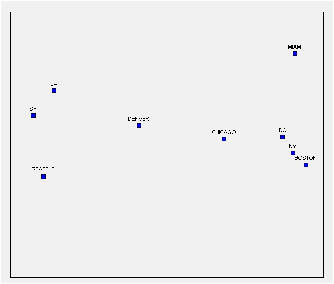
MDS can draw maps in any number of dimensions, but for the purposes of visualizing data on a screen or sheet of paper we use just one or two dimensions.
- distortion = stress (not fitting into the two-dimensional space)
- 0.2 = acceptance level for metric
- 0.12 = for non-metric (ordinal)
- the above case = .014
The first is that the axes are, in themselves, meaningless, and the second is that the orientation of the picture is arbitrary.
. . . two things to look for in interpreting an MDS picture: clusters and dimensions.
6.3. Correspondence analysis 
Correspondence analysis refers to a collection of closely related techniques, including optimal scaling and biplot analysis, which are used for a variety of purposes.
. . . primarily as a visualization applied to two-mode data.
. . . primarily as a visualization applied to two-mode data.
6.4. Hierarchical clustering 
Given a set of N actors to be clustered, and an N × N distance matrix, the basic process of Johnson’s (1967) hierarchical clustering is this:
- Start by assigning each item to its own cluster, so that if you have N items, you now have N clusters, each containing just one item. Let the distances between the clusters equal the distances between the items they contain.
- Find the closest pair of clusters and merge them into a single cluster, so that now you have one less cluster.
- Compute distances between the new cluster and each of the old clusters.'''
- Repeat steps 2 and 3 until all items are clustered into a single cluster of size N.
Step 3 can be done in different ways, which is what distinguishes
- single-link from
- complete-link (dia-meter, maximum) and
- average-link clustering.
- In single-link clustering (also called the nearest neighbor, the connectedness method and the minimum method), we consider the distance between one cluster and another cluster to be equal to the shortest distance from any member of one cluster to any member of the other cluster.
- In complete-link clustering (also called the diameter or maximum method), we consider the distance between one cluster and another cluster to be equal to the longest distance from any member of one cluster to any member of the other cluster.
- In average-link clustering, we consider the distance between one cluster and another cluster to be equal to the average distance from any member of one cluster to any member of the other cluster. More recently, Newman (2004) has introduced another criterion, which joins the pair of clusters that would maximize Q modularity, a measure of clustering quality.
7. 7 Visualization 
Data:  Roethlisberger & Dickson Bank Wiring Room (612 Bytes)
Data: Trade data (1.21 KB)
Data: Campnet data set (498 Bytes) as in Ch. 2
 Roethlisberger & Dickson Bank Wiring Room (612 Bytes)
Data:
 Trade data (1.21 KB)
Data:
 Campnet data set (498 Bytes) as in Ch. 2
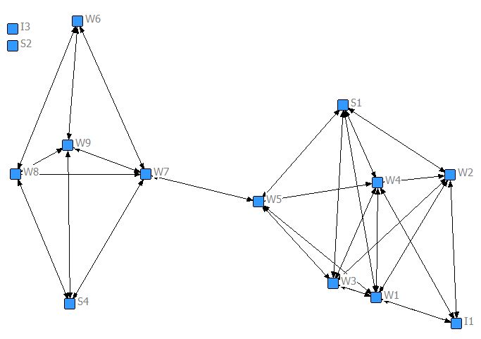
Netdraw output [JPG image (37.95 KB)]
NetDraw Layout -> Attributes at coordinates
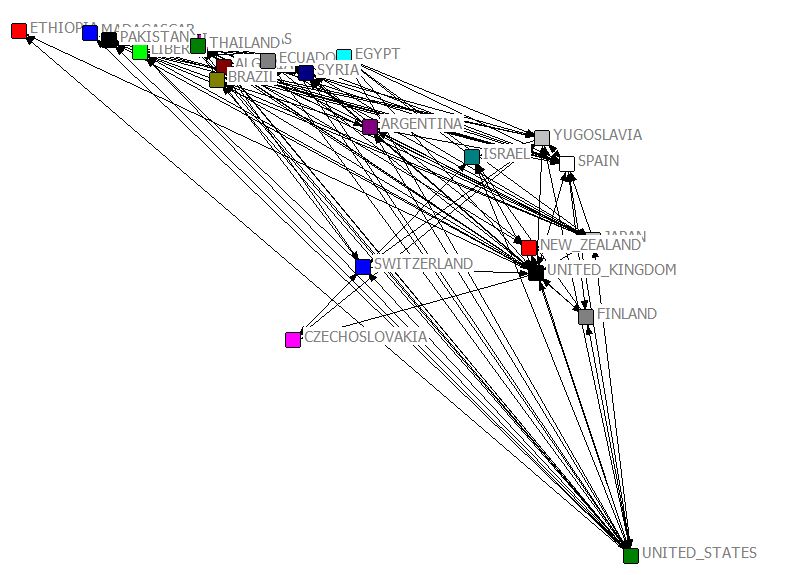
Using coordinates [JPG image (84.34 KB)]
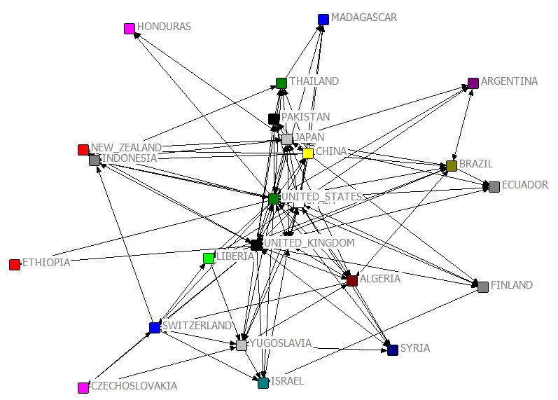
MDS [JPG image (81.82 KB)]
NetDraw Lighting bolt button
8. 8 Testing Hypotheses 
Permutation
. . . So you correlate the variables using your sample data, and get a value like 0.384. The classical significance test then tells you the probability of obtaining a correlation that large given that in the population the variables are actually independent (correlation zero). When this probability is really low (less than 0.05), we call it significant and are willing to claim that the variables are actually related in the population, and not just in your sample.
QAP CORRELATION
--------------------------------------------------------------------------------

Data Matrices:                          PADGB
                                        PADGM
# of Permutations:                      5000
Random seed:                            1
Method:                                 Fast: no missing values allowed


QAP results for PADGM * PADGB (5000 permutations)

                                 1         2         3         4         5         6         7         8
                         Obs Value Significa   Average   Std Dev   Minimum   Maximum Prop >= O Prop <= O
                         --------- --------- --------- --------- --------- --------- --------- ---------
    Pearson Correlation     0.3719    0.0008   -0.0004    0.0935   -0.1690    0.4395    0.0008    0.9998


QAP Correlations

               1     2
           PADGB PADGM
           ----- -----
  1 PADGB  1.000 0.372
  2 PADGM  0.372 1.000


QAP P-Values

               1     2
           PADGB PADGM
           ----- -----
  1 PADGB  0.000 0.001
  2 PADGM  0.001 0.000

QAP statistics saved as datafile QAP Correlation Results

----------------------------------------
Running time:  00:00:01
Output generated:  07 10 14 15:15:41
UCINET 6.511 Copyright (c) 1992-2012 Analytic Technologies
MULTIPLE REGRESSION QAP VIA DOUBLE DEKKER SEMI-PARTIALLING
--------------------------------------------------------------------------------

# of permutations:                      2000
Diagonal valid?:                        NO
Random seed:                            963
Dependent variable:                     KHTec-ADVICE
Partition variable (if any):
Predicted values:                       KHTec-ADVICE-mrpred (D:\Users\Hyo\OneDrive\Ucinet\Ch08\KHTec-ADVICE-mrpred
Residual values:                        KHTec-ADVICE-mrResid (D:\Users\Hyo\OneDrive\Ucinet\Ch08\KHTec-ADVICE-mrResid
Model fit stats:                        KHTec-ADVICE-mrfit (D:\Users\Hyo\OneDrive\Ucinet\Ch08\KHTec-ADVICE-mrfit
Model coefficients:                     KHTec-ADVICE-mrcoef (D:\Users\Hyo\OneDrive\Ucinet\Ch08\KHTec-ADVICE-mrcoef
Independent variables:                  D:\Users\Hyo\OneDrive\Ucinet\Ch08\KHTec-FRIENDSHIP
                                        D:\Users\Hyo\OneDrive\Ucinet\Ch08\KHTec-REPORTS_TO


MODEL FIT

                R-Square    Adj R-Sqr      P-Value          Obs        Perms
            ------------ ------------ ------------ ------------ ------------
      Model        0.063        0.059        0.000          420         2000


REGRESSION COEFFICIENTS

                         Un-Stdized Stdized Coef      P-value     As Large     As Small      Std Err
                       ------------ ------------ ------------ ------------ ------------ ------------
      KHTec-FRIENDSHIP      0.13582      0.11701      0.05097      0.05097      0.94953      0.08288
      KHTec-REPORTS_TO      0.47157      0.20177      0.00050      0.00050      1.00000      0.11902
             Intercept      0.39694      0.00000      0.00000      0.00000      0.00000      0.00000


-----------------------------------------
Running time: 00:00:01 seconds.
Output generated: 07 10 14 15:13:50
QAP LOGISTIC REGRESSION
--------------------------------------------------------------------------------

Dependent Variable:                     KHTec-ADVICE (D:\Users\Hyo\OneDrive\Ucinet\Ch08\KHTec-ADVICE
Independent Variables:                  D:\Users\Hyo\OneDrive\Ucinet\Ch08\KHTec-FRIENDSHIP
                                        D:\Users\Hyo\OneDrive\Ucinet\Ch08\KHTec-REPORTS_TO
# of permutations:                      1000
Random seed:                            1873119137
Statistics to track:                    T-Statistics
Data type:                              Non-Symmetric (directed)
Predicted values:                       KHTec-ADVICE-pred (D:\Users\Hyo\OneDrive\Ucinet\Ch08\KHTec-ADVICE-pred
Model fit stats:                        KHTec-ADVICE-fit (D:\Users\Hyo\OneDrive\Ucinet\Ch08\KHTec-ADVICE-fit
Model coefficients:                     KHTec-ADVICE-coef (D:\Users\Hyo\OneDrive\Ucinet\Ch08\KHTec-ADVICE-coef
Permutation history:                    history (D:\Users\Hyo\OneDrive\Ucinet\Ch08\history


Dependent variable: :                   KHTec-ADVICE

Overall fit of the logistic regression model

                          1         2         3         4         5
                         LL     R-Sqr       Sig       Obs     Perms
                  --------- --------- --------- --------- ---------
    1 Statistics:  -274.073     0.065     0.001       420      1000

1 rows, 5 columns, 1 levels.


LR Coefficients & Permutation Results (T-stats used in permutations)

                               1         2         3         4         5         6         7         8         9        10        11
                            Coef   OddsRat         T       Sig       Avg       Min       Max        SD     P(ge)     P(le)     Perms
                       --------- --------- --------- --------- --------- --------- --------- --------- --------- --------- ---------
    1        Intercept    -0.425     0.654    -3.666                                                                            1000
    2 KHTec-FRIENDSHIP     0.579     1.785     2.418     0.051     0.023    -1.244     0.948     0.345     0.051     0.950      1000
    3 KHTec-REPORTS_TO     3.059    21.306     2.956     0.001    -0.010    -1.521     3.059     0.540     0.001         1      1000

3 rows, 11 columns, 1 levels.


-----------------------------------------
Running time: 00:00:01 seconds.
Output generated: 07 10 14 15:21:24
. . . We shall examine the first two time periods to study reciprocity and transitivity. We are interested to know if new friendship ties formed in Week 1 are a result of reciprocity and/or transitivity of ties formed in week 0.
DL
N=17
FORMAT = FULLMATRIX DIAGONAL PRESENT
LEVEL LABELS:
"NEWC0"
DATA:
 0 0 0 0 0 0 0 0 0 0 1 0 1 0 0 0 1
 0 0 0 1 0 0 1 0 0 0 0 0 0 0 0 1 0
 0 0 0 0 0 0 0 0 0 0 1 1 0 0 0 0 1
 0 1 0 0 0 0 1 0 0 0 0 0 0 0 0 0 1
 0 0 0 0 0 0 0 0 0 0 1 1 0 0 0 0 1
 0 0 0 1 0 0 0 1 0 0 0 0 1 0 0 0 0
 0 0 0 1 0 0 0 0 0 0 0 1 0 0 0 0 1
 0 0 0 0 0 1 0 0 0 1 1 0 0 0 0 0 0
 0 0 0 0 0 0 0 0 0 0 1 1 0 0 0 0 1
 1 0 0 0 0 0 1 0 0 0 0 0 0 0 1 0 0
 0 0 0 0 0 0 0 0 1 0 0 1 0 0 0 0 1
 0 0 1 0 0 0 0 0 0 0 1 0 0 0 0 0 1
 1 0 0 0 0 1 0 0 0 0 0 0 0 0 1 0 0
 0 0 0 0 0 0 1 0 1 1 0 0 0 0 0 0 0
 0 0 0 0 1 0 0 0 0 1 1 0 0 0 0 0 0
 0 0 0 1 0 0 0 0 1 0 1 0 0 0 0 0 0
 0 0 0 1 0 0 0 0 1 0 0 1 0 0 0 0 0
DL
N=17
FORMAT = FULLMATRIX DIAGONAL PRESENT
LEVEL LABELS:
"NEWC1"
DATA:
 0 0 0 0 0 0 0 0 1 0 0 0 1 1 0 0 0
 0 0 0 1 0 0 1 0 0 0 0 0 0 0 0 0 1
 0 0 0 0 0 0 0 0 0 0 0 1 0 0 1 0 1
 0 1 0 0 0 0 0 0 1 0 0 0 0 0 0 0 1
 1 0 0 0 0 0 0 0 0 0 0 0 1 0 0 0 1
 1 0 0 0 0 0 0 0 1 0 0 0 1 0 0 0 0
 0 0 0 1 0 0 0 0 0 0 0 1 0 0 0 0 1
 0 0 0 0 0 1 0 0 0 1 0 0 1 0 0 0 0
 0 0 0 0 0 0 0 0 0 0 1 0 0 1 0 0 1
 1 0 0 0 0 0 1 0 0 0 0 0 1 0 0 0 0
 0 0 1 0 0 0 0 0 1 0 0 0 0 0 0 0 1
 0 0 1 0 0 0 1 0 1 0 0 0 0 0 0 0 0
 1 0 0 0 1 1 0 0 0 0 0 0 0 0 0 0 0
 0 0 0 1 0 0 1 0 1 0 0 0 0 0 0 0 0
 0 0 1 1 1 0 0 0 0 0 0 0 0 0 0 0 0
 0 0 0 0 0 0 0 0 1 0 1 0 0 0 0 0 1
 0 0 0 1 1 0 0 0 1 0 0 0 0 0 0 0 0
TRANSPOSE
--------------------------------------------------------------------------------

Input dataset:                          NEWC0D (D:\Users\Hyo\OneDrive\Ucinet\Ch08\NewFrat\NEWC0D)
Output dataset:                         NEWC0D-reciprocity (D:\Users\Hyo\OneDrive\Ucinet\Ch08\NewFrat\NEWC0D-reciprocity)


        1 2 3 4 5 6 7 8 9 1 1 1 1 1 1 1 1
        - - - - - - - - - - - - - - - - -
     1  0 0 0 0 0 0 0 0 0 1 0 0 1 0 0 0 0
     2  0 0 0 1 0 0 0 0 0 0 0 0 0 0 0 0 0
     3  0 0 0 0 0 0 0 0 0 0 0 1 0 0 0 0 0
     4  0 1 0 0 0 1 1 0 0 0 0 0 0 0 0 1 1
     5  0 0 0 0 0 0 0 0 0 0 0 0 0 0 1 0 0
     6  0 0 0 0 0 0 0 1 0 0 0 0 1 0 0 0 0
     7  0 1 0 1 0 0 0 0 0 1 0 0 0 1 0 0 0
     8  0 0 0 0 0 1 0 0 0 0 0 0 0 0 0 0 0
     9  0 0 0 0 0 0 0 0 0 0 1 0 0 1 0 1 1
    10  0 0 0 0 0 0 0 1 0 0 0 0 0 1 1 0 0
    11  1 0 1 0 1 0 0 1 1 0 0 1 0 0 1 1 0
    12  0 0 1 0 1 0 1 0 1 0 1 0 0 0 0 0 1
    13  1 0 0 0 0 1 0 0 0 0 0 0 0 0 0 0 0
    14  0 0 0 0 0 0 0 0 0 0 0 0 0 0 0 0 0
    15  0 0 0 0 0 0 0 0 0 1 0 0 1 0 0 0 0
    16  0 1 0 0 0 0 0 0 0 0 0 0 0 0 0 0 0
    17  1 0 1 1 1 0 1 0 1 0 1 1 0 0 0 0 0

Transposed matrix saved as dataset D:\Users\Hyo\OneDrive\Ucinet\Ch08\NewFrat\NEWC0D-reciprocity

----------------------------------------
Running time:  00:00:01
Output generated:  07 10 14 15:41:16
UCINET 6.511 Copyright (c) 1992-2012 Analytic Technologies
TRANSITIVIZE
--------------------------------------------------------------------------------


          1  2  3  4  5  6  7  8  9 10 11 12 13 14 15 16 17
         -- -- -- -- -- -- -- -- -- -- -- -- -- -- -- -- --
       1  0  0  0  1  0  1  0  0  1  0  1  1  1  0  1  0  1
       2  0  0  0  1  0  0  1  0  1  0  1  1  0  0  0  1  1
       3  0  0  0  1  0  0  0  0  1  0  1  1  0  0  0  0  1
       4  0  1  0  0  0  0  1  0  1  0  0  1  0  0  0  1  1
       5  0  0  1  1  0  0  0  0  1  0  1  1  0  0  0  0  1
       6  1  1  0  1  0  0  1  1  0  1  1  0  1  0  1  0  1
       7  0  1  1  1  0  0  0  0  1  0  1  1  0  0  0  0  1
       8  1  0  0  1  0  1  1  0  1  1  1  1  1  0  1  0  1
       9  0  0  1  1  0  0  0  0  0  0  1  1  0  0  0  0  1
      10  1  0  0  1  1  0  1  0  0  0  1  1  1  0  1  0  1
      11  0  0  1  1  0  0  0  0  1  0  0  1  0  0  0  0  1
      12  0  0  1  1  0  0  0  0  1  0  1  0  0  0  0  0  1
      13  1  0  0  1  1  1  0  1  0  1  1  0  0  0  1  0  1
      14  1  0  0  1  0  0  1  0  1  1  1  1  0  0  1  0  1
      15  1  0  0  0  1  0  1  0  1  1  1  1  0  0  0  0  1
      16  0  1  0  1  0  0  1  0  1  0  1  1  0  0  0  0  1
      17  0  1  1  1  0  0  1  0  1  0  1  1  0  0  0  0  0

17 rows, 17 columns, 1 levels.


-----------------------------------------
Running time: 00:00:01 seconds.
Output generated: 07 10 14 15:41:50
UCINET 6.511 Copyright (c) 1992-2012 Analytic Technologies
QAP LOGISTIC REGRESSION
--------------------------------------------------------------------------------

Dependent Variable:                     NEWC1D (D:\Users\Hyo\OneDrive\Ucinet\Ch08\NewFrat\NEWC1D
Independent Variables:                  D:\Users\Hyo\OneDrive\Ucinet\Ch08\NewFrat\NEWC0D
                                        D:\Users\Hyo\OneDrive\Ucinet\Ch08\NewFrat\NEWC0D-reciprocity
                                        D:\Users\Hyo\OneDrive\Ucinet\Ch08\NewFrat\NEWC0D-transitivity
# of permutations:                      10000
Random seed:                            2058888892
Statistics to track:                    T-Statistics
Data type:                              Non-Symmetric (directed)
Predicted values:                       NEWC1D-pred (D:\Users\Hyo\OneDrive\Ucinet\Ch08\NewFrat\NEWC1D-pred
Model fit stats:                        NEWC1D-fit (D:\Users\Hyo\OneDrive\Ucinet\Ch08\NewFrat\NEWC1D-fit
Model coefficients:                     NEWC1D-coef (D:\Users\Hyo\OneDrive\Ucinet\Ch08\NewFrat\NEWC1D-coef
Permutation history:                    history (D:\Users\Hyo\OneDrive\Ucinet\Ch08\NewFrat\history


Dependent variable: :                   NEWC1D

Overall fit of the logistic regression model

                           1          2          3          4          5
                          LL      R-Sqr        Sig        Obs      Perms
                  ---------- ---------- ---------- ---------- ----------
    1 Statistics:   -100.284      0.263      0.000        272      10000

1 rows, 5 columns, 1 levels.


LR Coefficients & Permutation Results (T-stats used in permutations)

                                   1          2          3          4          5          6          7          8          9         10         11
                                Coef    OddsRat          T        Sig        Avg        Min        Max         SD      P(ge)      P(le)      Perms
                          ---------- ---------- ---------- ---------- ---------- ---------- ---------- ---------- ---------- ---------- ----------
    1           Intercept     -2.764      0.063     -8.096                                                                                   10000
    2              NEWC0D      1.833      6.253      4.053      0.000     -0.007     -2.592      2.672      0.482      0.000      1.000      10000
    3  NEWC0D-reciprocity      0.806      2.239      1.943      0.012     -0.013     -1.868      1.160      0.369      0.012      0.988      10000
    4 NEWC0D-transitivity      0.923      2.517      1.982      0.045      0.001     -2.359      1.690      0.433      0.045      0.955      10000

4 rows, 11 columns, 1 levels.


-----------------------------------------
Running time: 00:00:03 seconds.
Output generated: 07 10 14 15:43:42
12. 12 Equivalence 
1 2 3 4 5 6 7 8 9 10 11 12 13 14 15 16 17 18

RO BO AM BE PE LO VI WI JO GR HU BO MA AL AM BA EL SI

-- -- -- -- -- -- -- -- -- -- -- -- -- -- -- -- -- --

ROMULAND 0 7 7 8 11 7 8 5 9 10 7 7 8 7 7 9 8 8

BONAVENTURE 7 0 5 8 12 8 7 8 10 12 9 8 9 8 9 11 10 10

AMBROSE 7 5 0 9 12 9 7 7 10 11 8 8 10 8 9 10 10 10

BERTHOLD 8 8 9 0 10 10 9 10 11 12 11 10 9 10 10 10 10 11

PETER 11 12 12 10 0 10 12 12 13 13 12 12 13 13 11 12 12 13

LOUIS 7 8 9 10 10 0 10 8 10 12 10 9 10 9 7 10 10 10

VICTOR 8 7 7 9 12 10 0 8 11 12 10 9 11 9 10 11 10 9

WINFRID 5 8 7 10 12 8 8 0 8 9 6 5 8 7 8 8 9 9

JOHN 9 10 10 11 13 10 11 8 0 10 10 10 11 10 9 11 11 11

GREGORY 10 12 11 12 13 12 12 9 10 0 9 9 11 10 11 9 12 12

HUGH 7 9 8 11 12 10 10 6 10 9 0 5 9 7 9 9 10 9

BONIFACE 7 8 8 10 12 9 9 5 10 9 5 0 7 5 9 9 9 9

MARK 8 9 10 9 13 10 11 8 11 11 9 7 0 6 9 9 9 9

ALBERT 7 8 8 10 13 9 9 7 10 10 7 5 6 0 9 9 9 9

AMAND 7 9 9 10 11 7 10 8 9 11 9 9 9 9 0 9 9 9

BASIL 9 11 10 10 12 10 11 8 11 9 9 9 9 9 9 0 7 9

ELIAS 8 10 10 10 12 10 10 9 11 12 10 9 9 9 9 7 0 5

SIMPLICIUS 8 10 10 11 13 10 9 9 11 12 9 9 9 9 9 9 5 0
1 2 3 4 5 6 7 8 9 10 11 12 13 14 15 16 17 18

RO BO AM BE PE LO VI WI JO GR HU BO MA AL AM BA EL SI

-- -- -- -- -- -- -- -- -- -- -- -- -- -- -- -- -- --

ROMULAND 0 7 7 8 11 7 8 5 9 10 7 7 8 7 7 9 8 8

BONAVENTURE 7 0 5 8 12 8 7 8 10 12 9 8 9 8 9 11 10 10

AMBROSE 7 5 0 9 12 9 7 7 10 11 8 8 10 8 9 10 10 10

BERTHOLD 8 8 9 0 10 10 9 10 11 12 11 10 9 10 10 10 10 11

PETER 11 12 12 10 0 10 12 12 13 13 12 12 13 13 11 12 12 13

LOUIS 7 8 9 10 10 0 10 8 10 12 10 9 10 9 7 10 10 10

VICTOR 8 7 7 9 12 10 0 8 11 12 10 9 11 9 10 11 10 9

WINFRID 5 8 7 10 12 8 8 0 8 9 6 5 8 7 8 8 9 9

JOHN 9 10 10 11 13 10 11 8 0 10 10 10 11 10 9 11 11 11

GREGORY 10 12 11 12 13 12 12 9 10 0 9 9 11 10 11 9 12 12

HUGH 7 9 8 11 12 10 10 6 10 9 0 5 9 7 9 9 10 9

BONIFACE 7 8 8 10 12 9 9 5 10 9 5 0 7 5 9 9 9 9

MARK 8 9 10 9 13 10 11 8 11 11 9 7 0 6 9 9 9 9

ALBERT 7 8 8 10 13 9 9 7 10 10 7 5 6 0 9 9 9 9

AMAND 7 9 9 10 11 7 10 8 9 11 9 9 9 9 0 9 9 9

BASIL 9 11 10 10 12 10 11 8 11 9 9 9 9 9 9 0 7 9

ELIAS 8 10 10 10 12 10 10 9 11 12 10 9 9 9 9 7 0 5

SIMPLICIUS 8 10 10 11 13 10 9 9 11 12 9 9 9 9 9 9 5 0
13.1. 7. Equivalence 
Use the Davis data
Use the two output files, with the original data file
Tools -> Similarities & Distances---
input: davis
output: davis-Mat-C

Matches . . . . Cols
---
input: davis
output: davis-Mat-R

Matches . . . . Rows
---
Use the two output files, with the original data file
Network -> Cohesion -> Density with Group
input: davis
row partition: davis-Mat-R
columns partion: davis-Mat-C


![[http]](/imgs/http.png)
