Sampling Distribution

I mentioned in the earlier article that the standard error is actually standard deviation of sampling distribution. I would feel safe when I say standard deviation since I covered the concept already. However, I thought you might feel uneasy about "sampling distribution," which may lead you all to a confusion in understanding standard error concept. If so, the article was not good enough. But, I mention about the concept (sampling distribution) implicitly without providing the definitions. So, I want to talk more about the concepts of "central tendency," "sampling distribution" and "standard error."

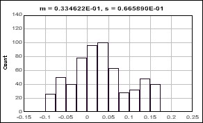
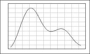
Do you remember you heard something like "no matter how the population is distributed, the statistics from the infinite numbers of samples will have normal distribution characteristics?" Suppose that the below graph show how a population is distributed (The first one is histogram, the second is distribution graph).

Certainly, you see that the distribution is not normal.

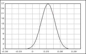
Now suppose that you took a sample from this population and recorded the mean of the sample. And suppose that you kept doing this about 1000 times. How do you think the curve of the graph look a like? Remember that you kept the means of the 10000 samples. The graph looks like the below -- normally distributed curve. Again, this is obtained from numerous numbers of sample means -- this is not about the sample itself.

This can be called normal curve of mean (x bar). And this distribution is called sampling distribution because the distribution graph is obtained by keeping sampling for a very very large number of times. Weiss and Leets (1998) say "The sampling distribution is a theoretical distribution that is a fundamental basis for inferential statistics" (p.71).

This sampling distribution has several interesting characteristics:
(1) `mu_(bar(x))=mu` (2) `sigma_(bar(x)=sigma/sqrt(n)`. We all know what the sign means, the symbols are "m " and "s " in Greek, representing "mean" and "standard deviation." The subscribed letter is for identification -- who's the owner of the Greek characters? That is, The first one is mean of means (x bar), the second one is standard deviation of sampling means, (x bar). So, we can interpret them as: (1) The mean of sampling distribution is about the same as that of population. (2) The standard deviation of sampling distribution is about "standard deviation of the population/square root of sample size."

The second is also called "standard error of the mean." Oops, it is been covered in previous writing, but was different from this one... We are talking about sampling distribution of mean, not sampling distribution of probability. They are same thing, but obtained via different methods (they share the same idea, though).

For the reference, the standard deviation of sampling distribution of probability was,
`sigma_(bar(p))=sqrt(p*q/n)` As you see, they share the same Greek letter, "s," "standard deviation." Strangely, they are called the standard error of the mean or the standard error of the probability.

What is this used for? At the bottom line, this is very important to do any kind of statistical (inferential) analysis. Illustration of this idea requires us to expand our thoughts a bit more, however. This is directly related to the t-test and z-test (Therefore, I strongly recommend to read "z" score section in the textbook). I will save this kind of example for the next writing.

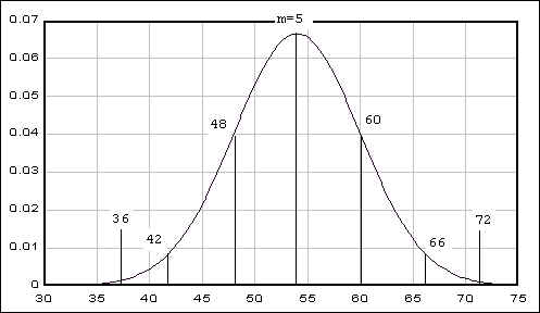
Instead, I want to talk about an example which is related to the exact above concept. Suppose that you are a member of a consumer group. The director called you -- since you have taken statistics and media research course at Rutgers -- and asked you to test a brand of battery. She wanted to know whether the battery life, which the manufacturer has announced to the public, holds the truth. The manufacturer has claimed that the lengths of life of its best battery has a mean of 54 months and a standard deviation of 6 months. The director told you to send a sample of 50 of the batteries.

Immediately, you draw a picture in your mind even before you get the sample set:

You are expecting that the picture represents the entire population of the batteries: their mean is about 54; about 68% of the batteries will last long between 48-60 months; 42-66 months for the 95%; 36-72 months for the 99%. And you are expecting this claim holds the truths.

You can also imagine how the sampling distribution -- again, the ones from the means obtained from imaginary sampling -- should look like based on the information. First, you know that the mean of means (the mean of the sampling distribution of means) is the same as that of the population. And the standard deviation of the sampling distribution is standard deviation of population divided by square root of sample size. That is,

, which is known as 54, and
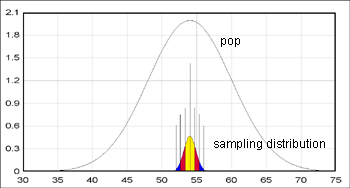
`sigma_(bar(x))=sigma/sqrt(n)=6/sqrt(50)`, which is about 0.85 month. These two again gives you a picture of sampling distribution. which will look like the below graph.

The inner distribution line is "sampling distribution of means" line, which shares the same mean and different (narrow -- always the case) standard deviation (0.85, in this case). The ranges of the corresponding standard deviation unit is:

	minimum	maximum
mean (+-) 1s (68%)	53.15	54.85	yellow
mean (+-) 2s (95%)	52.3	55.7	yellow	red
mean (+-) 3s (99%)	51.45	56.55	yellow	red	blue

Keep in mind that the numbers are representing the mean of your sample, not the individual sample score. Now, suppose that the mean of you particular sample set (n=50) turned out to be 52. How should you think of the mean of the sample? ----- According to the table, the score 52 resides outside of the second raw range. That is, your mean is outside of the range in which 95% of means of sample means can be found. In other words, this is a rare extreme case, if you have to believe the manufacturer's claim. In 95 out of 100 cases, the means are supposed to be found in between 52.3 to 55.7. And this case (mean=52) is supposed to be the five out of 100 cases. Therefore, your sample shows that the information which the manufacturer gives us is unlikely true. Maybe the realistic battery life is a bit shorter than that it advertise. You also acknowledge that the chance of your claim to be false (accusing the manufacturer) is about five out of 100 cases. (This means that even though you find the mean of battery life in the sample set is 52, the sample might have been from such a rare case (one of 5 out of 100 cases). Your director will get your report tomorrow morning and send the story to the major media hoping that they will listen to it.

Reference

Weiss, A. J., & Leets, L. L. (1998). Introduction to Statistics for the Social Sciences (2nd ed.). New York, NY: McGraw Hill.

CategoryResearchMethods
CategoryStatistics